Image processing, Computer Vision and Computer Graphics#
Image Processing: Image Processing is the field of enhancing the images by tuning many parameter and features of the images. So Image Processing is the subset of Computer Vision. Here, transformations are applied to an input image and the resultant output image is returned. Some of these transformations are- sharpening, smoothing, stretching etc. Now, as both the fields deal with working in visuals, i.e., images and videos, there seems to be lot of confusion about the difference about these fields of computer science.
Computer Vision: In Computer Vision, computers or machines are made to gain high-level understanding from the input digital images or videos with the purpose of automating tasks that the human visual system can do. It uses many techniques and Image Processing is just one of them.
Computer graphics
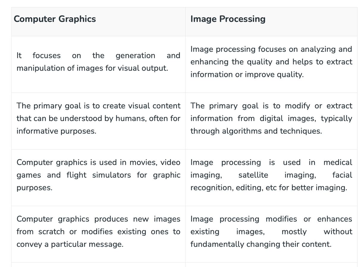
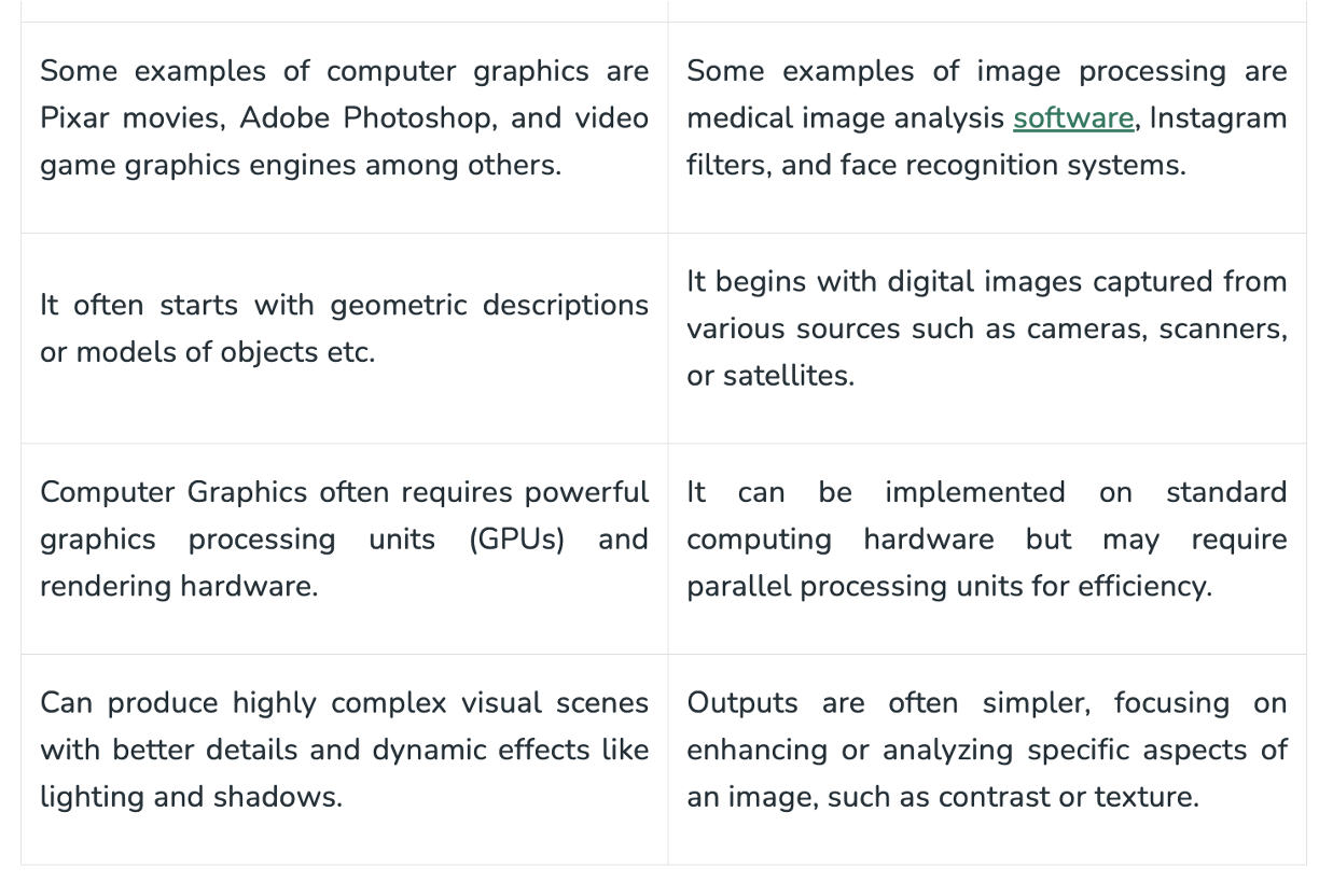
In Computer Graphics are introduced as drawings or any type of sketch that can represent some meaningful information in the form of pictures. Computer graphics is used widely in the software and computer field when there is a set of images that needs to be created or manipulated such as in digital films, the entertainment industry, or digital photography.
Image processing and computer vision
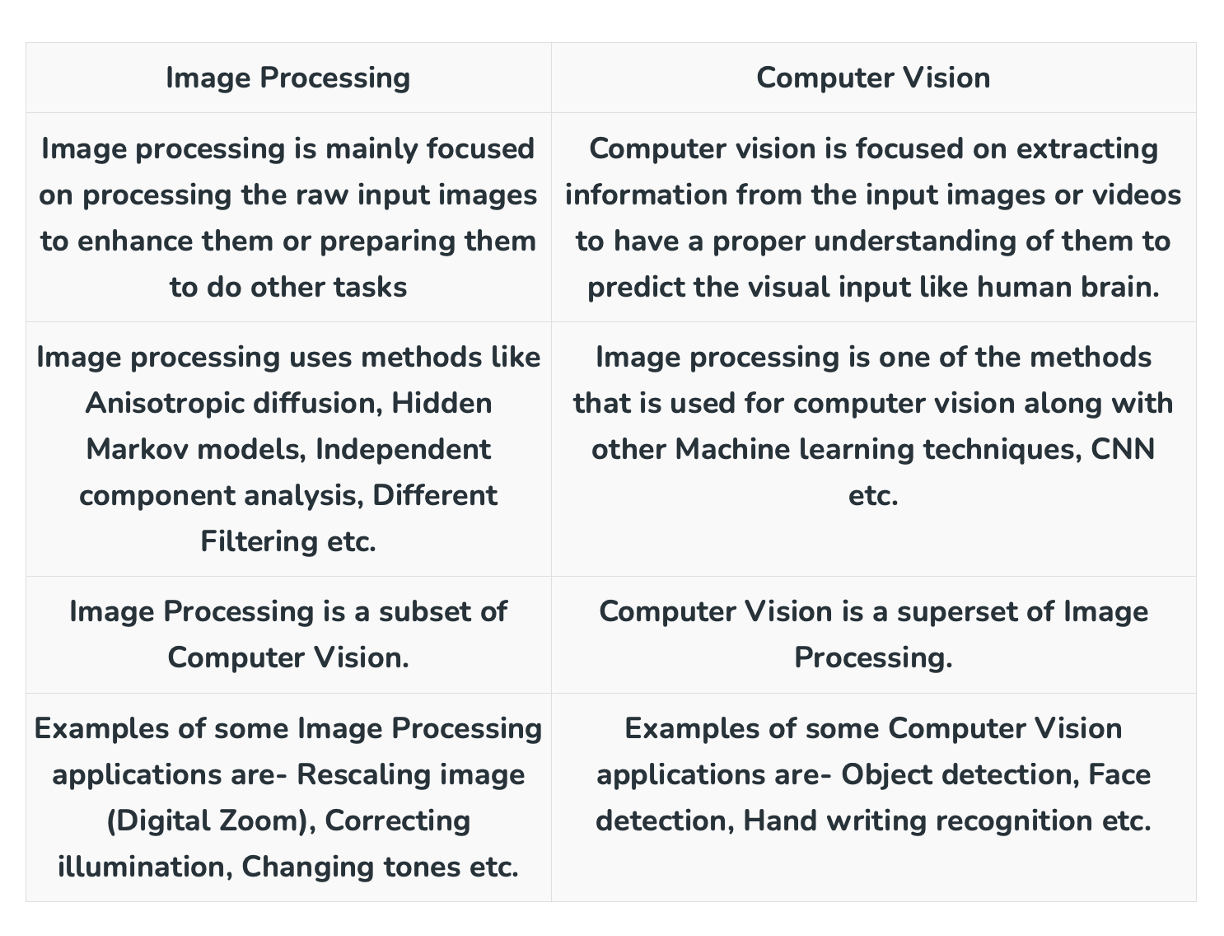
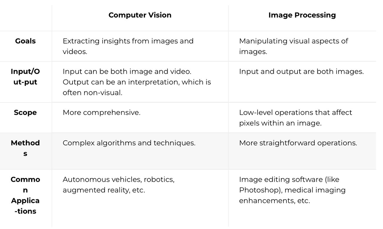
Image processing and computer graphics
Computational imaging
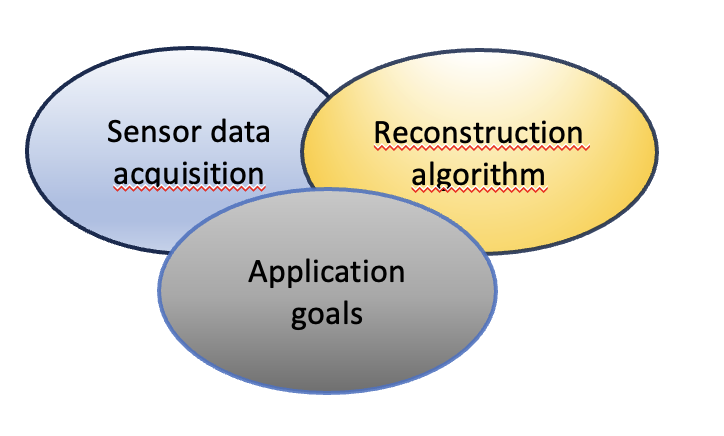
Computational algorithms are essential to convert data to images.
Contrary to popular believes, sensors almost never directly generate usable images.
Real imaging systems require that raw sensors date be processed using algorithms to form the resulting images.
Why a math course on Computational Imaging in the Computer Science LM?
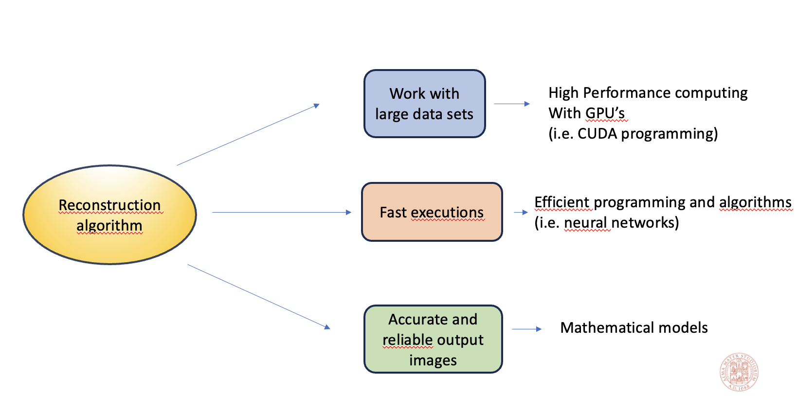
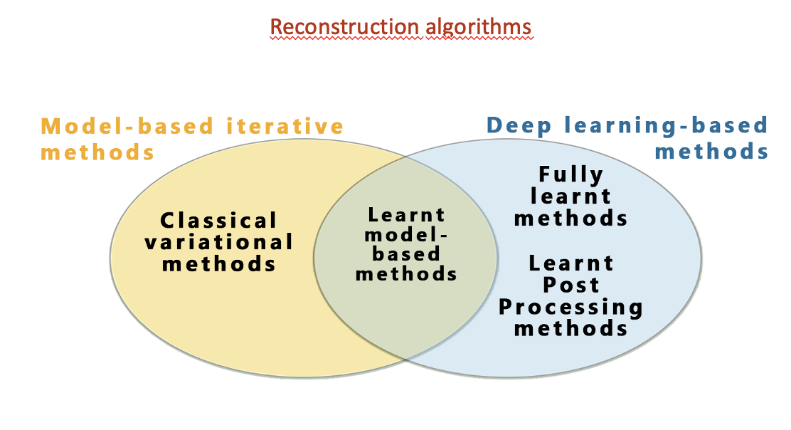
Organization of the CI course
Module I:
Introduction to computational imaging (CI) CI as inverse problem Model-based reconstruction methods
Module II:
Introduction to different types of neural networks in imaging Deep learning based reconstruction methods Learnt model based reconstruction methods (a mention)
Both with examples python programs.
The digital image#
A continuous (or analogue) grayscale image is a function \(f:\Omega \subset R^2 \rightarrow R\)
A discrete (or digital) image A is a matrix of size M xN obtained by discretinzing the function f.
The intersection between a row and a column is called pixel
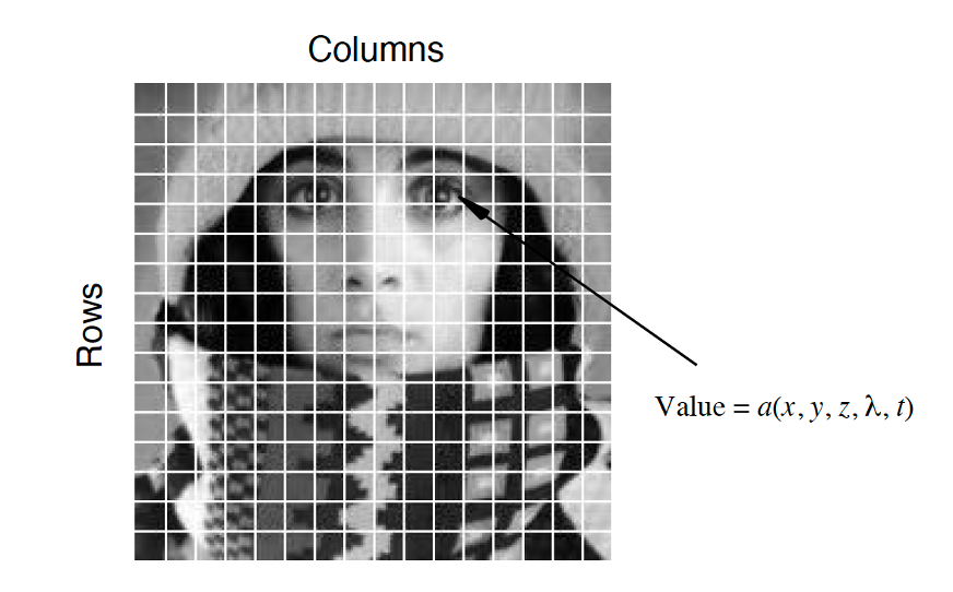
The value assigned to every pixel is the average brightness in the pixel rounded to the nearest integer value. The process of representing the amplitude of the 2D signal at a given coordinate as an integer value with L different gray levels is usually referred to as amplitude quantization or simply quantization.
In the case of color images, three values are associated to each pixel, for example in the R(red)G(green)B(blue) (RGB) scale. Many techniques developed for the single channel image are repeated on the three channels .
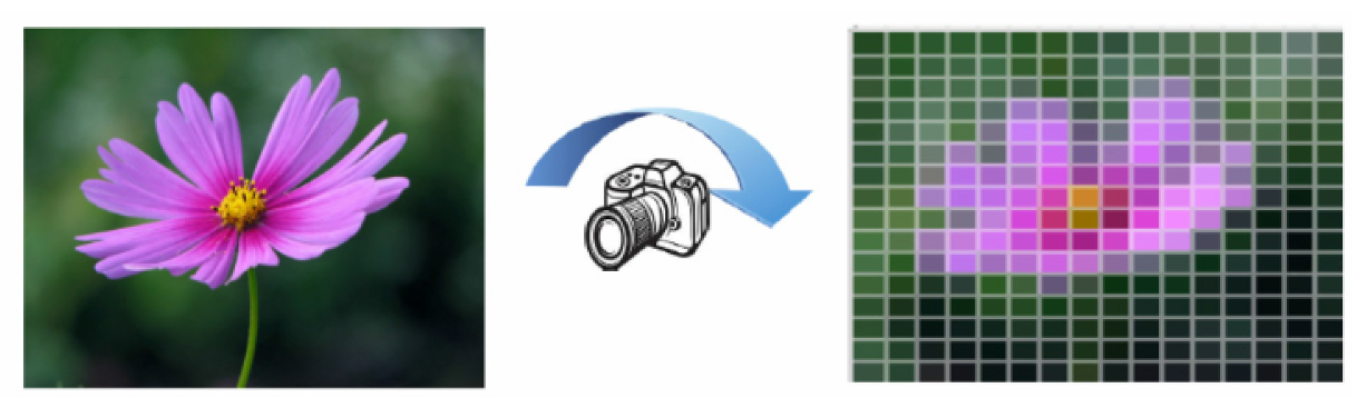
Example of RGB channels of a color image.
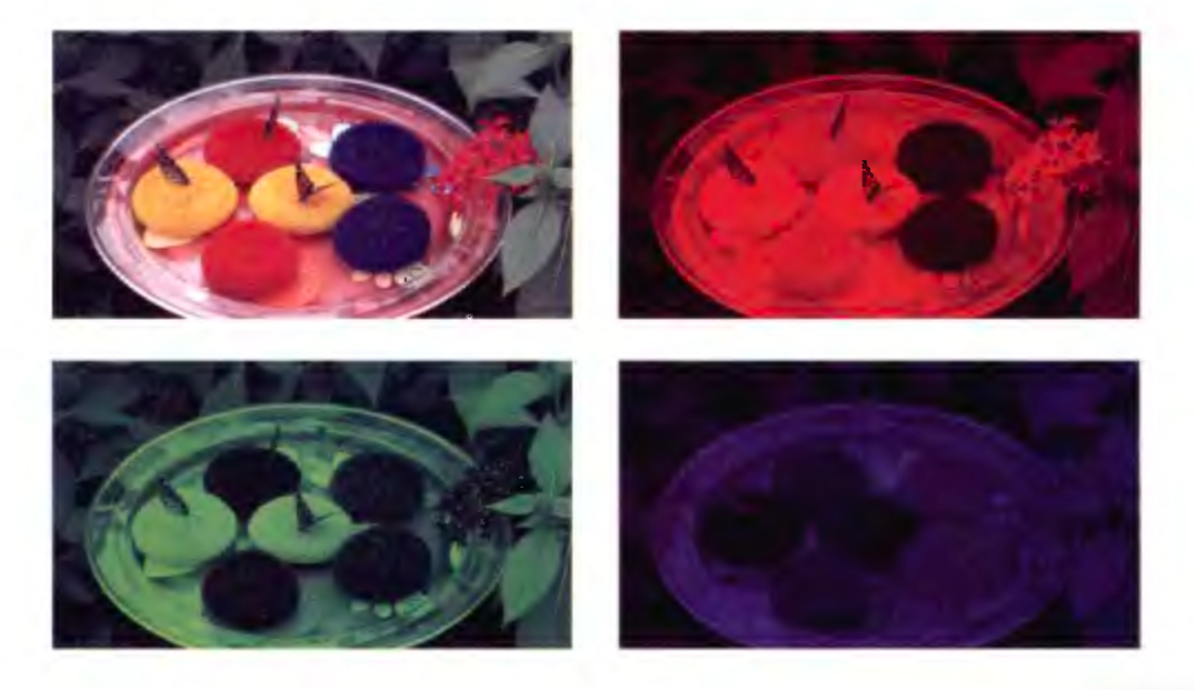
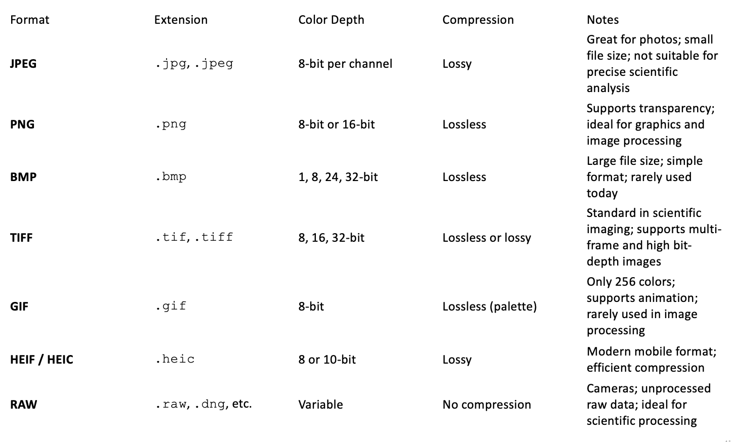
Image file formats
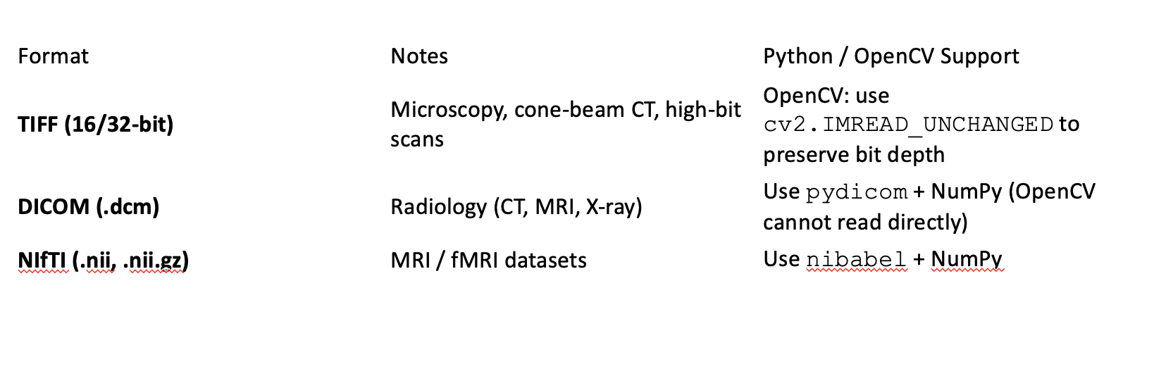
A DICOM file (Digital Imaging and Communications in Medicine) is a standard format used for medical images (CT, MRI, ultrasound, X-ray, etc.) that combines both the image and clinical/technical information in a single file. It’s not just an image—it’s a structured container.
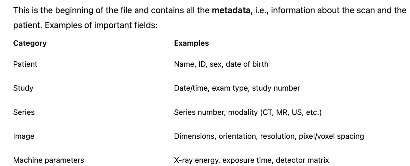
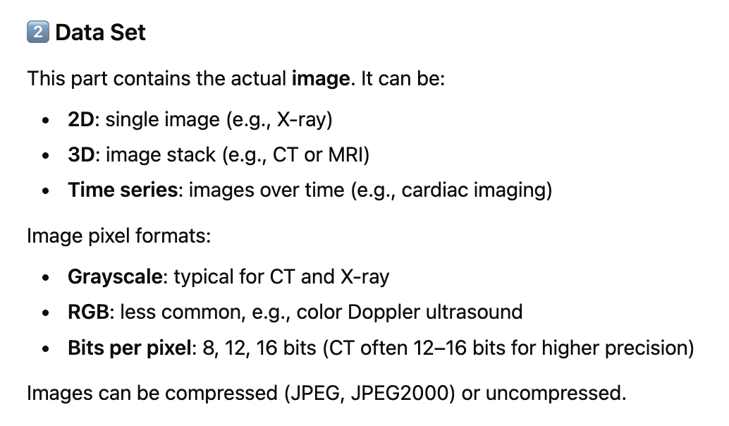
In python, we can use the pydicom library to explore both metadata and the image in the dicom file.
How to read images in Python#

Open CV
Computer vision + fast processing.
Filters, edge detection, warping, feature detection, registration, calibration, etc. Very fast (C++ underneath). Excellent for numerical pipelines.
How it represents the image: numpy.ndarray Color channels: default is BGR (not RGB) → classic source of confusion. Data types: handles uint8, uint16, and float very well.
Pros:
Very complete for image processing
High performance
Huge number of algorithms Cons:
BGR vs RGB confusion
imshow requires a GUI (often does not work in notebooks)
Matplotlib
Visualization and plotting (not an “image processing library”).
Used for: Displaying images in notebooks Creating figures with overlays, colormaps, colorbars, ROIs, etc. Perfect for scientific 2D/3D images (slices, heatmaps)
How it represents the image: numpy.ndarray Colors: expects RGB (or grayscale) Data types: often works best with normalized float values or uint8; special care needed for 16-bit images.
Pros:
Ideal for debugging and reports
Works everywhere (including Jupyter) Cons:
Not designed for “serious” image processing (although some things can be done)
Slower than OpenCV for certain operations
Pillow (PIL)
I/O and “image-style” manipulations (photography/graphics).
What it is used for:
Open/save images
Resize, crop, rotate
Draw text, ….
Very convenient for working with “standard” PNG/JPEG/TIFF images How it represents the image: PIL.Image.Image object You can convert it to NumPy with np.array(img). Colors: typically RGB (or L, RGBA, etc.)
Pros:
Simple and clean API
Excellent for common formats and basic operations Cons:
Less suitable for advanced computer vision
With scientific 16-bit/float images it can be more “delicate” (depends on the format)
ImageIO
Easy reading/writing of many formats (including stacks).
What it is used for:
Convenient for saving GIFs/videos or reading image sequences How it represents the image: numpy.ndarray Colors: usually RGB (depends on the format/plugin)
Pros:
Very simple for NumPy-based I/O
Excellent for multi-page / stack TIFF files
Cons:
Not a processing library: mainly focused on I/O
Different backends/plugins → sometimes different behaviors
import numpy as np

# use OpenCV

import cv2

#img_cv = cv2.imread("peppers_color.tif")
img_cv = cv2.imread("images.jpeg")
print("OpenCV:")
print(type(img_cv))
print(" shape:", img_cv.shape)
print(" dtype:", img_cv.dtype)
print(" min/max:", img_cv.min(), img_cv.max())


# OpenCV visualization (desktop only)
# cv2.imshow("OpenCV image", img_cv)
# cv2.waitKey(0)
# cv2.destroyAllWindows()

# Save the image
cv2.imwrite("images_cv.jpeg", img_cv)
OpenCV:
<class 'numpy.ndarray'>
 shape: (451, 679, 3)
 dtype: uint8
 min/max: 0 255
True
#Use ImageIO

import imageio.v2 as imageio

#img_io = imageio.imread("peppers_color.tif")
img_io = imageio.imread("images.jpeg")
print("ImageIO:")
print(type(img_io))
print(" shape:", img_io.shape)
print(" dtype:", img_io.dtype)
print(" min/max:", img_io.min(), img_io.max())


# --- Check the difference between the two arrays  (convert OpenCV in RGB) ---
img_cv_rgb = cv2.cvtColor(img_cv, cv2.COLOR_BGR2RGB)

diff = np.abs(img_cv_rgb.astype(int) - img_io.astype(int))
print("\nMaximum difference between OpenCV (converted  in RGB) and  Imageio:", diff.max())

# Save the image

#Make sure your array dtype is np.uint8 for normal 8-bit images.

# If you have floating-point arrays (0–1), scale them to 0–255 first:

#image_uint8 = (image_float * 255).astype(np.uint8)
imageio.imwrite("output_image_imageio.jpeg", img_io)
ImageIO:
<class 'numpy.ndarray'>
 shape: (451, 679, 3)
 dtype: uint8
 min/max: 0 255

Maximum difference between OpenCV (converted  in RGB) and  Imageio: 0
# use pyplot

import matplotlib.pyplot as plt

#img_plt = plt.imread("peppers_color.tif")
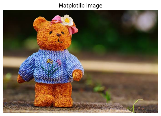
img_plt = plt.imread("images.jpeg")
print("Matplotlib:")
print(" shape:", img_plt.shape)
print(" dtype:", img_plt.dtype)
print(" min/max:", img_plt.min(), img_plt.max())


# Matplotlib visualization
plt.imshow(img_plt)
plt.title("Matplotlib image")
plt.axis('off')
plt.show()

# Save
plt.imsave("image_plt.jpeg", img_plt)

# if the image is grayscale:
#plt.imsave("image_plt_bn.jpeg", img_plt,cmap="gray")
Matplotlib:
 shape: (451, 679, 3)
 dtype: uint8
 min/max: 0 255
# Dicom file
import pydicom

# Read  dicom file
ds = pydicom.dcmread("proj.dcm")

# Show the main metadata
print(ds)

# Show the image
plt.figure()
plt.imshow(ds.pixel_array, cmap='gray')
plt.show()

#ds1 = pydicom.dcmread("reco.dcm")

# Show the main metadata
#print(ds1)
Dataset.file_meta -------------------------------
(0002,0000) File Meta Information Group Length  UL: 206
(0002,0001) File Meta Information Version       OB: b'\x00\x01'
(0002,0002) Media Storage SOP Class UID         UI: Digital Mammography X-Ray Image Storage - For Processing
(0002,0003) Media Storage SOP Instance UID      UI: 2.16.840.1.113669.632.25.1.103374.20240502120725128.10.3.5
(0002,0010) Transfer Syntax UID                 UI: Explicit VR Little Endian
(0002,0012) Implementation Class UID            UI: 1.2.276.0.7230010.3.0.3.6.3
(0002,0013) Implementation Version Name         SH: 'OFFIS_DCMTK_363'
-------------------------------------------------
(0008,0005) Specific Character Set              CS: 'ISO_IR 100'
(0008,0008) Image Type                          CS: ['ORIGINAL', 'PRIMARY', '', '', '']
(0008,0016) SOP Class UID                       UI: Digital Mammography X-Ray Image Storage - For Processing
(0008,0018) SOP Instance UID                    UI: 2.16.840.1.113669.632.25.1.103374.20240502120725128.10.3.5
(0008,0020) Study Date                          DA: '20240502'
(0008,0021) Series Date                         DA: '20240502'
(0008,0022) Acquisition Date                    DA: '20240502'
(0008,0023) Content Date                        DA: '20240502'
(0008,0030) Study Time                          TM: '090232'
(0008,0031) Series Time                         TM: '120715'
(0008,0032) Acquisition Time                    TM: '120725'
(0008,0033) Content Time                        TM: '120725'
(0008,0050) Accession Number                    SH: ''
(0008,0060) Modality                            CS: 'MG'
(0008,0068) Presentation Intent Type            CS: 'FOR PROCESSING'
(0008,0070) Manufacturer                        LO: 'IMS GIOTTO S.p.A.'
(0008,0090) Referring Physician's Name          PN: ''
(0008,1010) Station Name                        SH: 'GIOTTO CLASS'
(0008,1050) Performing Physician's Name         PN: ''
(0008,1070) Operators' Name                     PN: ''
(0008,1090) Manufacturer's Model Name           LO: 'GIOTTO CLASS'
(0008,2218)  Anatomic Region Sequence  1 item(s) ----
   (0008,0100) Code Value                          SH: 'T-04000'
   (0008,0102) Coding Scheme Designator            SH: 'SRT'
   (0008,0104) Code Meaning                        LO: 'Breast'
   ---------
(0008,3010) Irradiation Event UID               UI: 2.16.840.1.113669.632.25.1.103374.20240502120715307.8
(0010,0010) Patient's Name                      PN: 'DBT^31 PROJ'
(0010,0020) Patient ID                          LO: 'MADAVERO'
(0010,0030) Patient's Birth Date                DA: '19840328'
(0010,0040) Patient's Sex                       CS: 'F'
(0010,1010) Patient's Age                       AS: '040Y'
(0010,1020) Patient's Size                      DS: None
(0010,1030) Patient's Weight                    DS: None
(0018,0015) Body Part Examined                  CS: 'BREAST'
(0018,0060) KVP                                 DS: '27'
(0018,1000) Device Serial Number                LO: '103374'
(0018,1020) Software Versions                   LO: 'Raffaello 4.19.8.0 - IMSProc 4.17.3.2 - Tiziano 4.15.0.3'
(0018,1030) Protocol Name                       LO: 'Mammography'
(0018,1110) Distance Source to Detector         DS: '688.9'
(0018,1111) Distance Source to Patient          DS: '672.0'
(0018,1114) Estimated Radiographic Magnificatio DS: '1.000'
(0018,1147) Field of View Shape                 CS: 'RECTANGLE'
(0018,1149) Field of View Dimension(s)          IS: [297, 233]
(0018,1150) Exposure Time                       IS: '38'
(0018,1151) X-Ray Tube Current                  IS: '104'
(0018,1152) Exposure                            IS: '4'
(0018,1153) Exposure in uAs                     IS: '4050'
(0018,1160) Filter Type                         SH: 'STRIP'
(0018,1164) Imager Pixel Spacing                DS: [0.0829, 0.0829]
(0018,1166) Grid                                CS: 'NONE'
(0018,1190) Focal Spot(s)                       DS: '0.3'
(0018,1191) Anode Target Material               CS: 'TUNGSTEN'
(0018,11A0) Body Part Thickness                 DS: '40'
(0018,11A2) Compression Force                   DS: '9.8'
(0018,11A4) Paddle Description                  LO: '24x30'
(0018,1405) Relative X-Ray Exposure             IS: '2075'
(0018,1508) Positioner Type                     CS: 'MAMMOGRAPHIC'
(0018,1510) Positioner Primary Angle            DS: '0'
(0018,1511) Positioner Secondary Angle          DS: '0'
(0018,1530) Detector Primary Angle              DS: '0'
(0018,1531) Detector Secondary Angle            DS: '0.907889'
(0018,5101) View Position                       CS: 'CC'
(0018,7001) Detector Temperature                DS: '32'
(0018,7004) Detector Type                       CS: 'DIRECT'
(0018,7005) Detector Configuration              CS: 'AREA'
(0018,700A) Detector ID                         SH: 'AP01-23387'
(0018,700C) Date of Last Detector Calibration   DA: '20240418'
(0018,701A) Detector Binning                    DS: [1, 1]
(0018,7020) Detector Element Physical Size      DS: [0.085, 0.085]
(0018,7022) Detector Element Spacing            DS: [0.085, 0.085]
(0018,702B) Detector Manufacturer's Model Name  LO: 'SCREEN+'
(0018,7050) Filter Material                     CS: 'SILVER'
(0018,7052) Filter Thickness Minimum            DS: '0.05'
(0018,7054) Filter Thickness Maximum            DS: '0.05'
(0018,7060) Exposure Control Mode               CS: 'AUTOMATIC'
(0018,7062) Exposure Control Mode Description   LT: Array of 184 elements
(0018,8151) X-Ray Tube Current in uA            DS: '104400'
(0018,9559) Positioner Primary Angle Direction  CS: 'CW'
(0020,000D) Study Instance UID                  UI: 2.16.840.1.113669.632.25.1.103374.20240502090232863.1
(0020,000E) Series Instance UID                 UI: 2.16.840.1.113669.632.25.1.103374.20240502120715244.2.5
(0020,0010) Study ID                            SH: '581-193'
(0020,0011) Series Number                       IS: '18'
(0020,0013) Instance Number                     IS: '10'
(0020,0020) Patient Orientation                 CS: ['P', 'L']
(0020,0052) Frame of Reference UID              UI: 2.16.840.1.113669.632.25.1.103374.20240502120715286.6
(0020,0062) Image Laterality                    CS: 'R'
(0020,1040) Position Reference Indicator        LO: ''
(0028,0002) Samples per Pixel                   US: 1
(0028,0004) Photometric Interpretation          CS: 'MONOCHROME1'
(0028,0010) Rows                                US: 3580
(0028,0011) Columns                             US: 2812
(0028,0100) Bits Allocated                      US: 16
(0028,0101) Bits Stored                         US: 13
(0028,0102) High Bit                            US: 12
(0028,0103) Pixel Representation                US: 0
(0028,0120) Pixel Padding Value                 US: 7500
(0028,0121) Pixel Padding Range Limit           US: 1952
(0028,0300) Quality Control Image               CS: 'YES'
(0028,0301) Burned In Annotation                CS: 'NO'
(0028,1040) Pixel Intensity Relationship        CS: 'LIN'
(0028,1041) Pixel Intensity Relationship Sign   SS: 1
(0028,1052) Rescale Intercept                   DS: '0'
(0028,1053) Rescale Slope                       DS: '1'
(0028,1054) Rescale Type                        LO: 'US'
(0028,1300) Breast Implant Present              CS: 'NO'
(0028,1350) Partial View                        CS: 'NO'
(0028,2110) Lossy Image Compression             CS: '00'
(0040,0244) Performed Procedure Step Start Date DA: '20240502'
(0040,0245) Performed Procedure Step Start Time TM: '090232'
(0040,0253) Performed Procedure Step ID         SH: '20231333'
(0040,0254) Performed Procedure Step Descriptio LO: ''
(0040,0314) Half Value Layer                    DS: '0.518'
(0040,0316) Organ Dose                          DS: '0.00062'
(0040,0318) Organ Exposed                       CS: 'BREAST'
(0040,0555)  Acquisition Context Sequence  0 item(s) ----
(0040,8302) Entrance Dose in mGy                DS: '0.179'
(0040,8303) Entrance Dose Derivation            CS: 'IAK'
(0054,0220)  View Code Sequence  1 item(s) ----
   (0008,0100) Code Value                          SH: 'R-10242'
   (0008,0102) Coding Scheme Designator            SH: 'SRT'
   (0008,0104) Code Meaning                        LO: 'cranio-caudal'
   (0054,0222)  View Modifier Code Sequence  0 item(s) ----
   ---------
(1269,0010) Private Creator                     LO: 'Raffaello Biopsy Private Code'
(1269,1001) Private tag data                    IS: '0'
(1271,0010) Private Creator                     LO: 'Raffaello Mammography Private Code'
(1271,1020) Private tag data                    IS: '3'
(1271,1021) Private tag data                    IS: '2'
(1271,1022) Private tag data                    IS: '0'
(1271,1025) Private tag data                    IS: '0'
(1271,1038) Private tag data                    LO: 'YES'
(1271,1039) Private tag data                    US: [268, 268]
(1271,1040) Private tag data                    US: [536, 536]
(1271,1041) Private tag data                    LO: ['CURRENT', 'STANDARD']
(1271,1053) Private tag data                    LO: '1.00'
(1271,1054) Private tag data                    IS: '0'
(1271,1055) Private tag data                    LO: '1952'
(1271,1070) Private tag data                    DS: '648.8'
(1271,1071) Private tag data                    DS: '0.000'
(1271,1072) Private tag data                    DS: '0.000'
(1271,1073) Private tag data                    DS: '0.000'
(1271,1074) Private tag data                    IS: '1792'
(1271,1075) Private tag data                    IS: '0'
(1271,1076) Private tag data                    DS: '0.964'
(1271,1077) Private tag data                    DS: '0.964'
(1271,1078) Private tag data                    DS: '0.964'
(1271,1079) Private tag data                    IS: '10'
(1271,1080) Private tag data                    IS: '21'
(1271,1082) Private tag data                    IS: '1'
(1271,1083) Private tag data                    LO: ''
(1271,1084) Private tag data                    LO: ''
(1271,1086) Private tag data                    LT: Array of 73 elements
(1271,1087) Private tag data                    IS: '6'
(1271,1088) Private tag data                    IS: '0'
(1271,1091) Private tag data                    LO: '1.4'
(1271,1093) Private tag data                    IS: '0'
(1271,1097) Private tag data                    IS: '7500'
(1271,1098) Private tag data                    IS: '2'
(1271,1099) Private tag data                    IS: '2'
(1271,109A) Private tag data                    IS: '2'
(1271,109B) Private tag data                    IS: '2'
(1271,10A1) Private tag data                    US: 0
(1271,10A4) Private tag data                    LO: ''
(1271,10A5) Private tag data                    SS: 0
(1271,10B2) Private tag data                    DS: '-0.90789'
(2050,0020) Presentation LUT Shape              CS: 'INVERSE'
(7FE0,0010) Pixel Data                          OW: Array of 20133920 elements
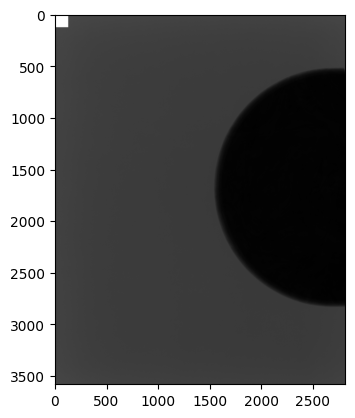
Image compression#
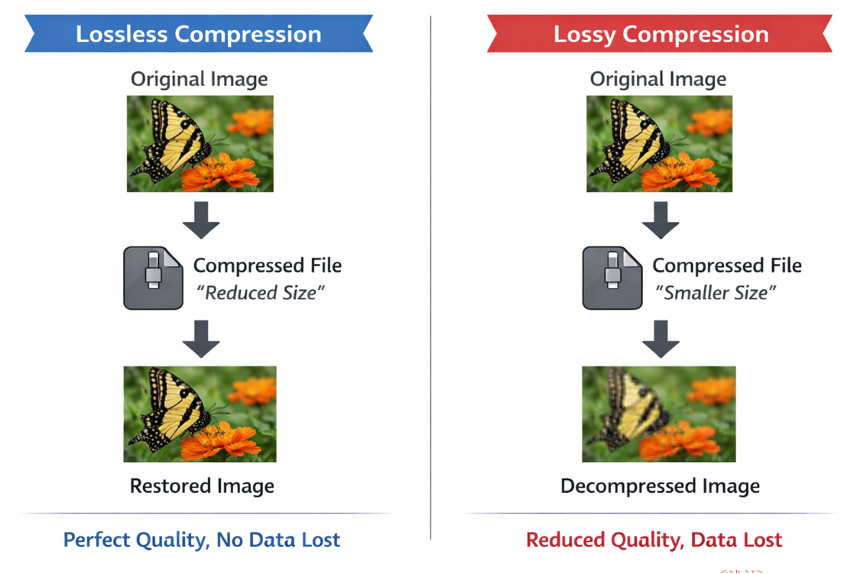
Image compression is the process of reducing the file size of an image while trying to preserve as much of its quality as possible.
Why compress images?
To save storage space.
To speed up loading times (e.g., on websites or apps).
To reduce bandwidth usage when transmitting images over the internet. Basically, compression tries to store the same image with fewer bits.
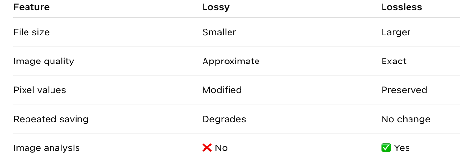
There are two main types: lossless and lossy.
Lossless compression
Definition: Compression where no information is lost. The original image can be perfectly reconstructed from the compressed file.
Lossy compression
Definition: Compression where some information is discarded, and the original image cannot be perfectly recovered.
Digital images#
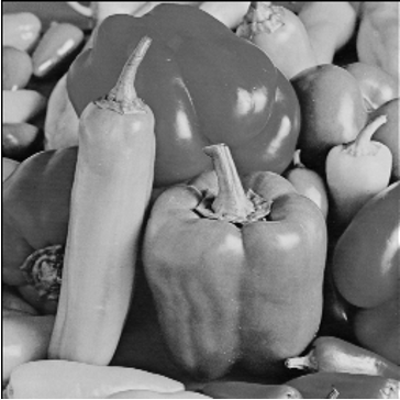
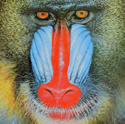
Photographic images
Medical images
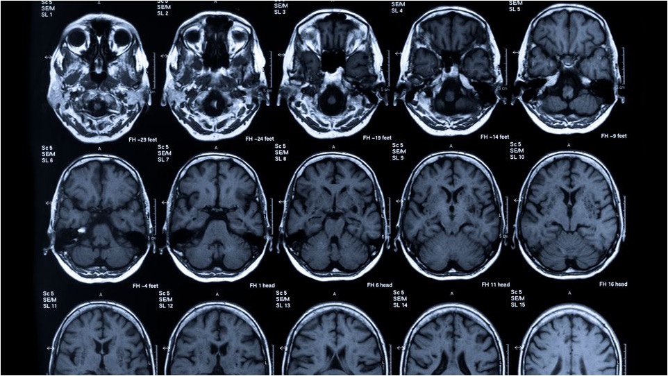
Medical images are usually gray-scale images, where the pixel intensity represents the density of the material (or the attenuation coefficient, which is proportional to the density).
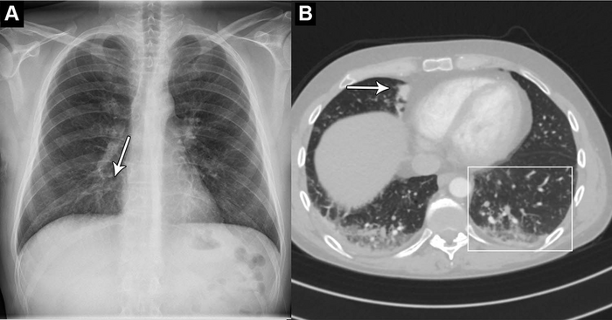
Medical images can be stacked in a 2D+1 volume, which represents the 3D object.
Microscopy images
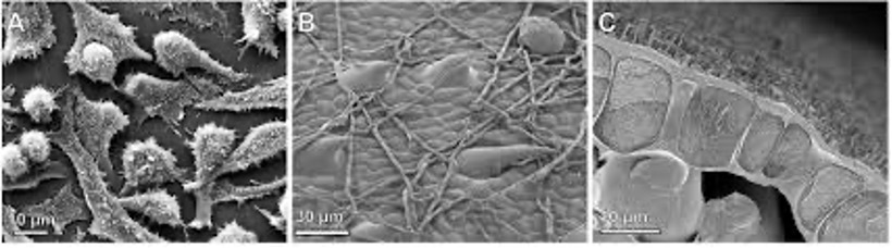
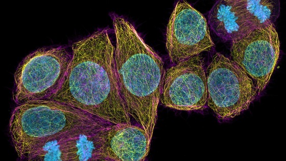
Images from microscopy can be quite different, since there are different kinds of microscopies. They can be grayscale or color images.
Thermal images
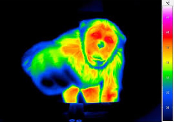
Thermal images are one-channel images, where the pixel intensity represents the temperature. They are usually displayed in a color scale, not in grayscale, to evidence hotter and colder regions.
Hyperspectral images
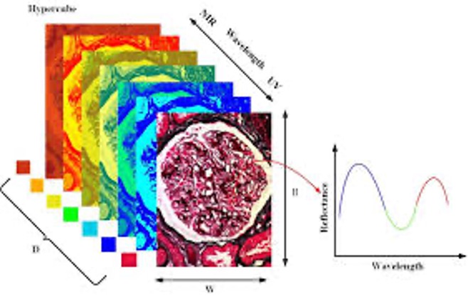
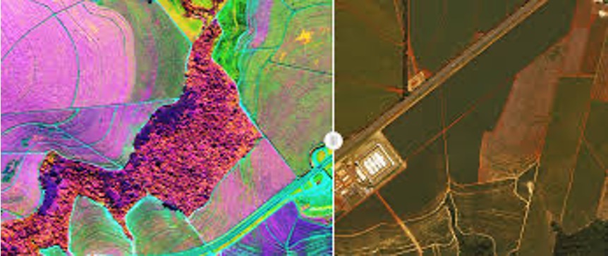
Hyperspectral images are tensor images where three dimensions (for color images) contain the color and one more dimensions contains spectral information. Examples of spectral information:
Earth information: infrared or NIR values
Thermal information: temperature
Environmental information: air quality, kind of soil
Physics information: wavelength ….