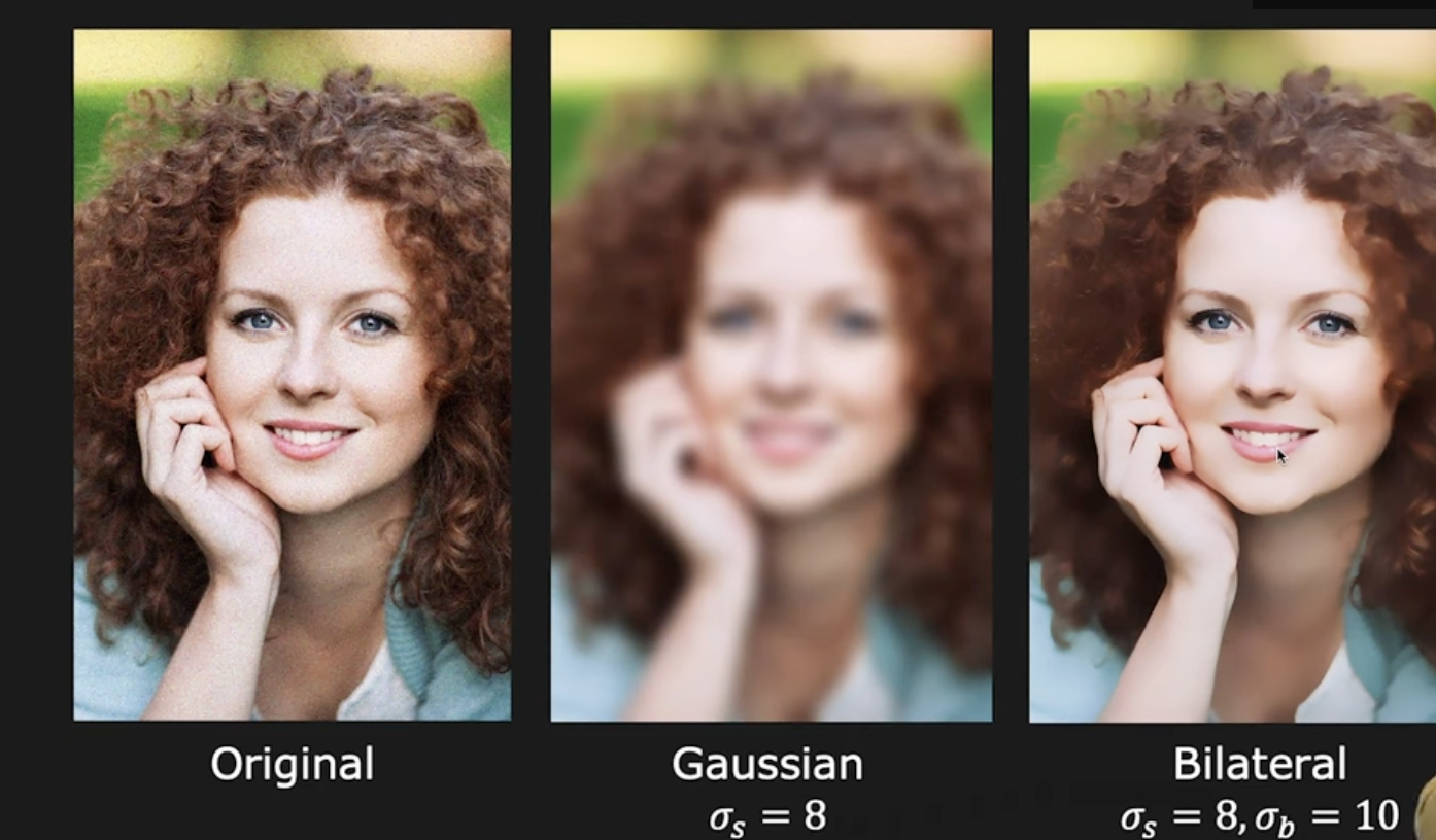
Image filtering#
Definition. A filter is an operation or system that selectively modifies a signal by enhancing, attenuating, or removing certain components, while leaving others relatively unchanged. Those components can be defined in terms of:
frequency (most common)
space (image filtering)
time (temporal filtering)
Mathematically: A filter is a function or operator \(H\) that transforms an input signal \(x\) into an output signal \(y\) as:
Think of a filter as a gate:
lets some information pass
blocks or weakens the rest
Examples:
sunglasses → filter light intensity
audio equalizer → filters sound frequencies
Common types of filters in the frequency domain:
Low-pass filter: passes low frequencies and suppresses high frequencies Effect: smoothing / blurring
High-pass filter: passes high frequencies and suppresses low frequencies Effect: edge enhancement / detail
Band-pass filter: passes only a range of frequencies
Filters in images
Low frequencies → global structure, smooth regions
High frequencies → edges, textures, noise That’s why:
blurring = low-pass filtering
edge detection = high-pass filtering
Linear Shift Invariant Systems (LSIS)#
Linear Shift Invariant Systems (LSIS) are very important in image processing.
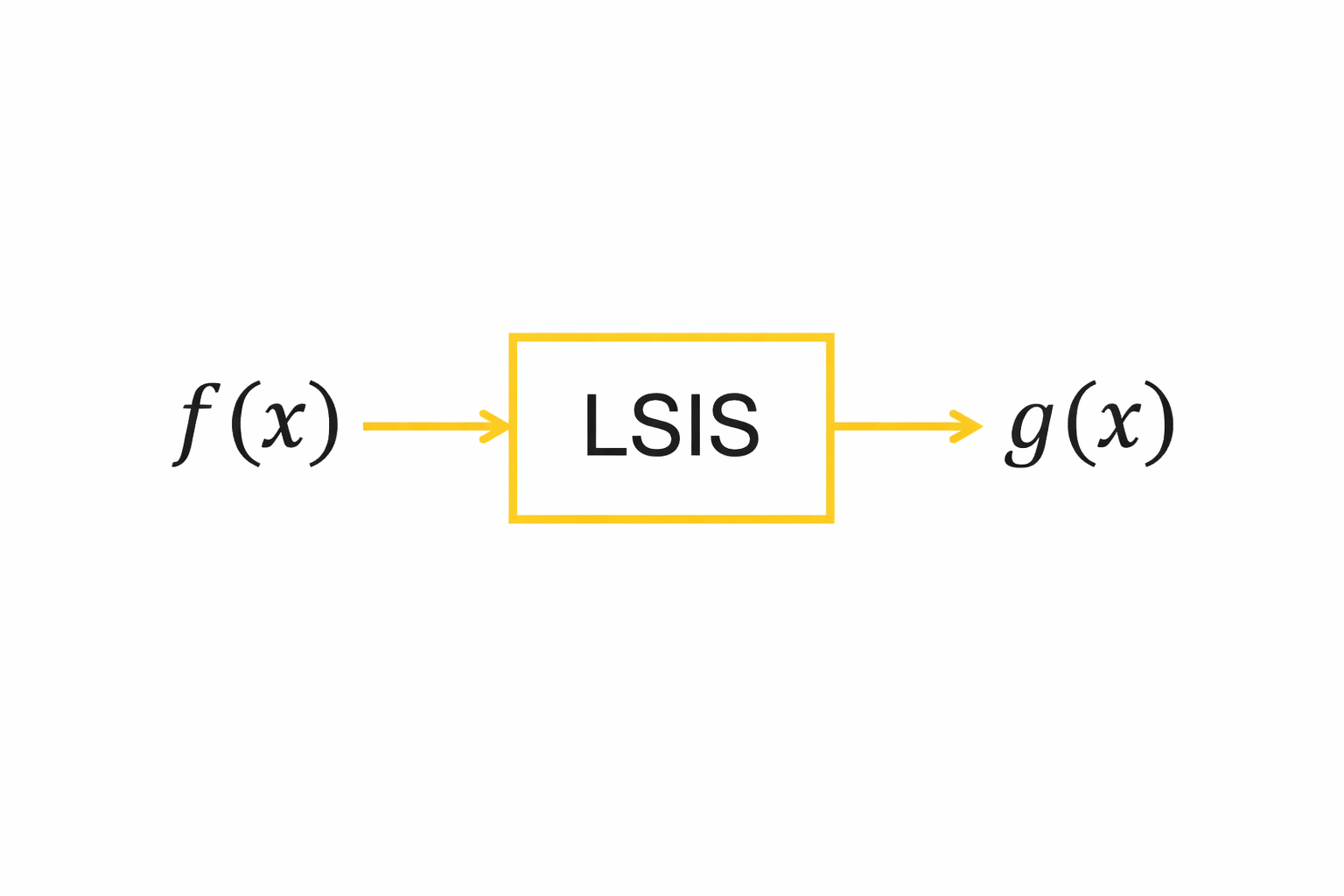
We consider first one dimensional signals.The extension to two dimensional signals, i.e. images, will be simple.
It leads to lots of useful image processing algorithms, beacuse many tasks in image processing can be described by LSIS.
What is a LSIS?
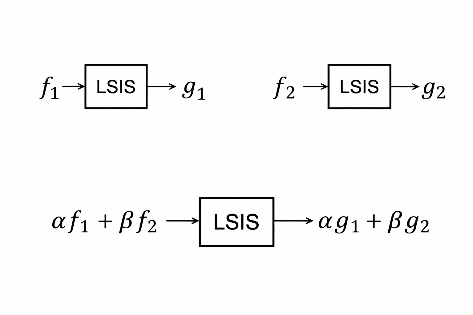
Property 1. Linearity:
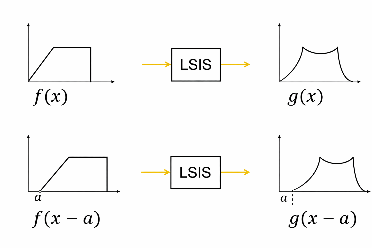
Property 2. Shift invariance:
Why are LSIS important?
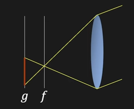
If the object moves far from the lens, the new image is obtained by applying a LSIS to the previous one.
The defocused image \(g\) is the processed version of the image \(f\).
linearity: brightness variation
shift invariance scene movement in \(f\) has the same movements in \(g\).
Convolution#
Convolutions of two 1D functions \(f(x)\) and \(h(x)\):
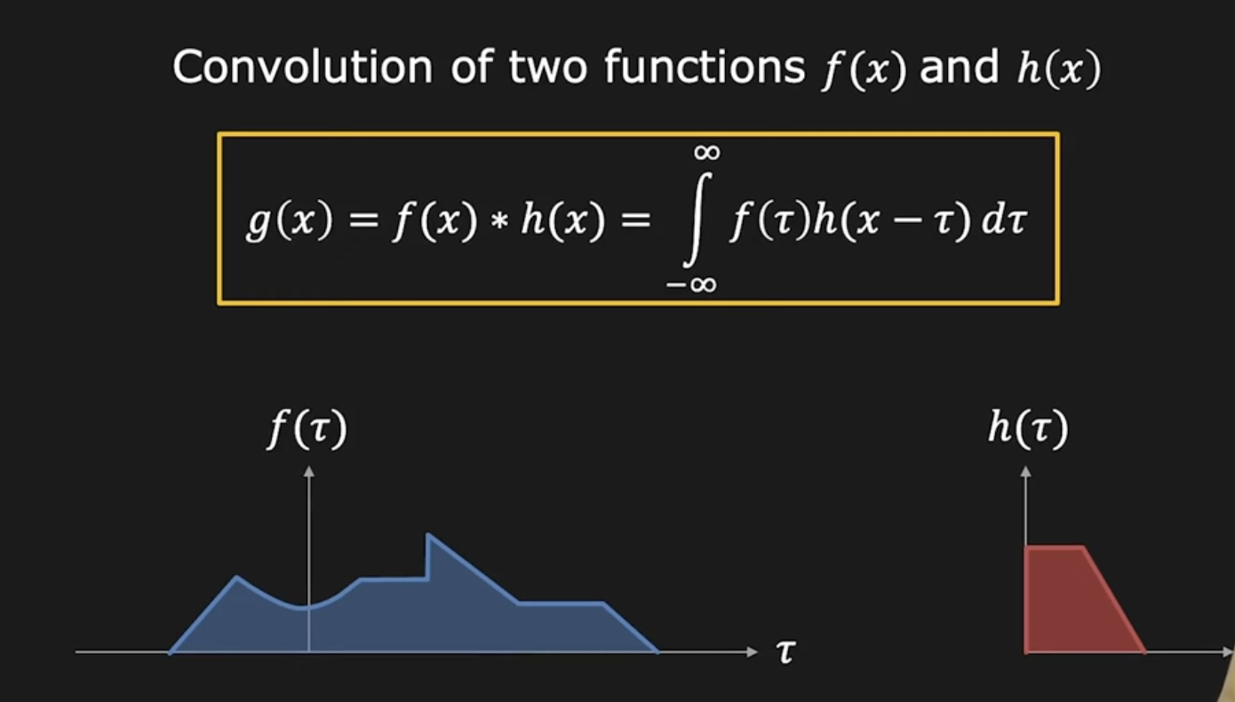
We follow the steps.
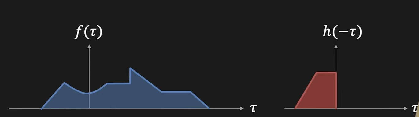
Fig. 1 Step 1- Draw f and h#
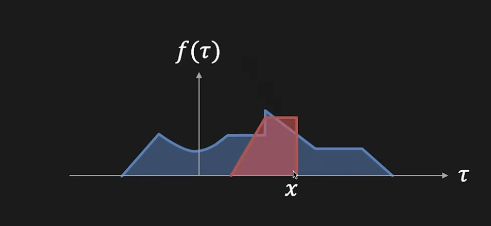
Fig. 2 Step 2 -#
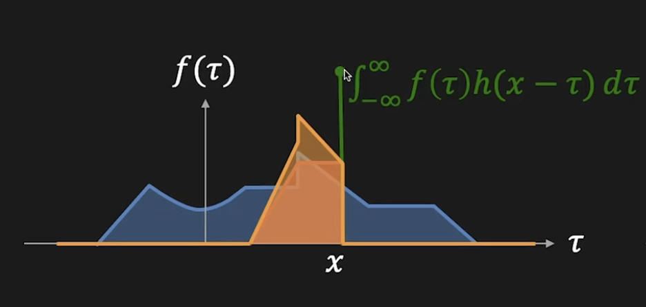
Fig. 3 Step 3- multiply f and h and compute the integral.#
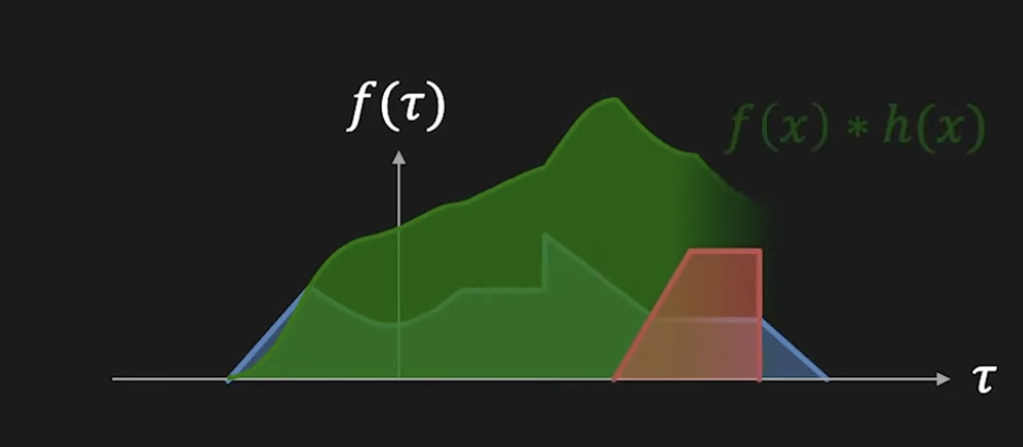
Fig. 4 Step 4- repeat Step 3 for all the x in the domain.#
Any LSIS implies convolution and whenever you perform a convolution you have a LSIS.
Examples:
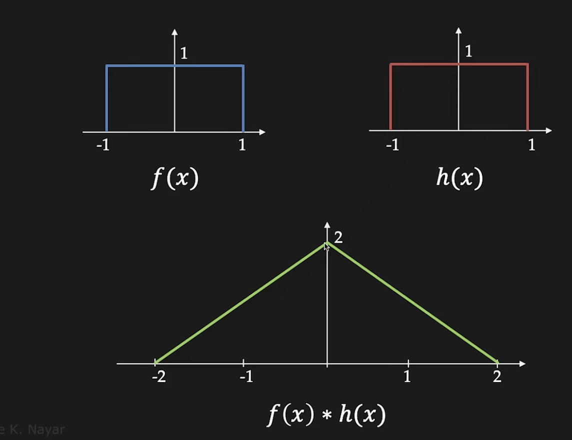
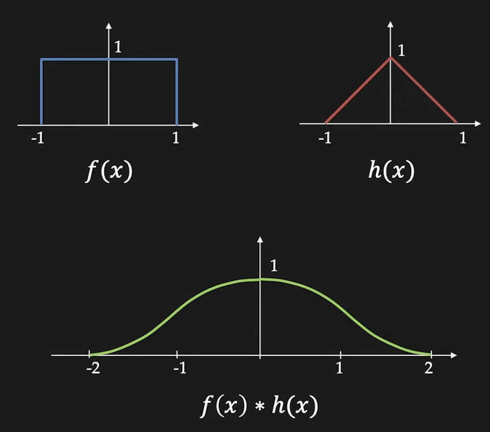
When you perform a convolution, the result is a function that satisfy linearity and shift inversion.
Linearity $\(g_1(x)=\int f_1(\tau)h(x-\tau)d\tau, \ \ g_2(x)=\int f_2(\tau)h(x-\tau)d\tau \)$
then: $\(\int (\alpha f_1(\tau) + \beta f_2(\tau)) h(x-\tau)d\tau=\)\( \)\(= \alpha \int f_1(\tau) h(x-\tau)d\tau+ \beta \int f_2(\tau) h(x-\tau)d\tau\)\( \)\(=\alpha g_1(x)+\beta g_2(x)\)$
Shift invariance $\(g(x)=\int f(\tau)h(x-\tau)d\tau\)\( Then: \)\(\int f(\tau -a) h(x-\tau)d\tau=\int f(\mu)h(x-a-\mu)d\mu=g(x-a)\)$
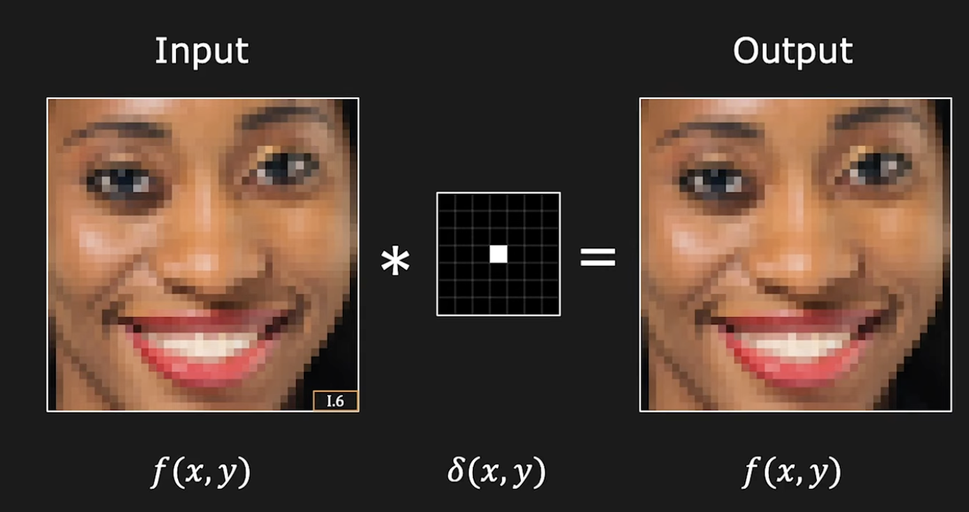
The unit of the convolution operator is the unit impulse function
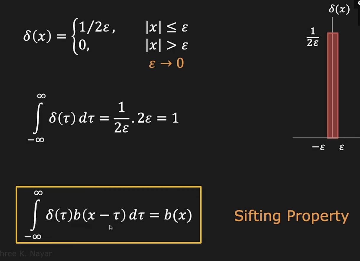
If you convolve it with any function \(f\), the result is \(f\).
Properties of Convolution
Commutative: ab=ba
Associative: a*(bc)=(ab)*c
2D Convolution and linear image filters#
In case of 2D functions the convolution is extended as: $\(g(x,y)=\int \int f(\tau,\mu)h(x-\tau,y-\mu) d\tau d\mu\)$
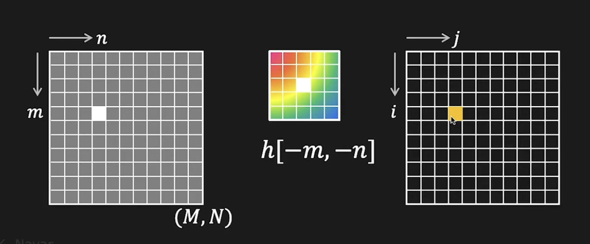
In the discrete case, for images, we have:
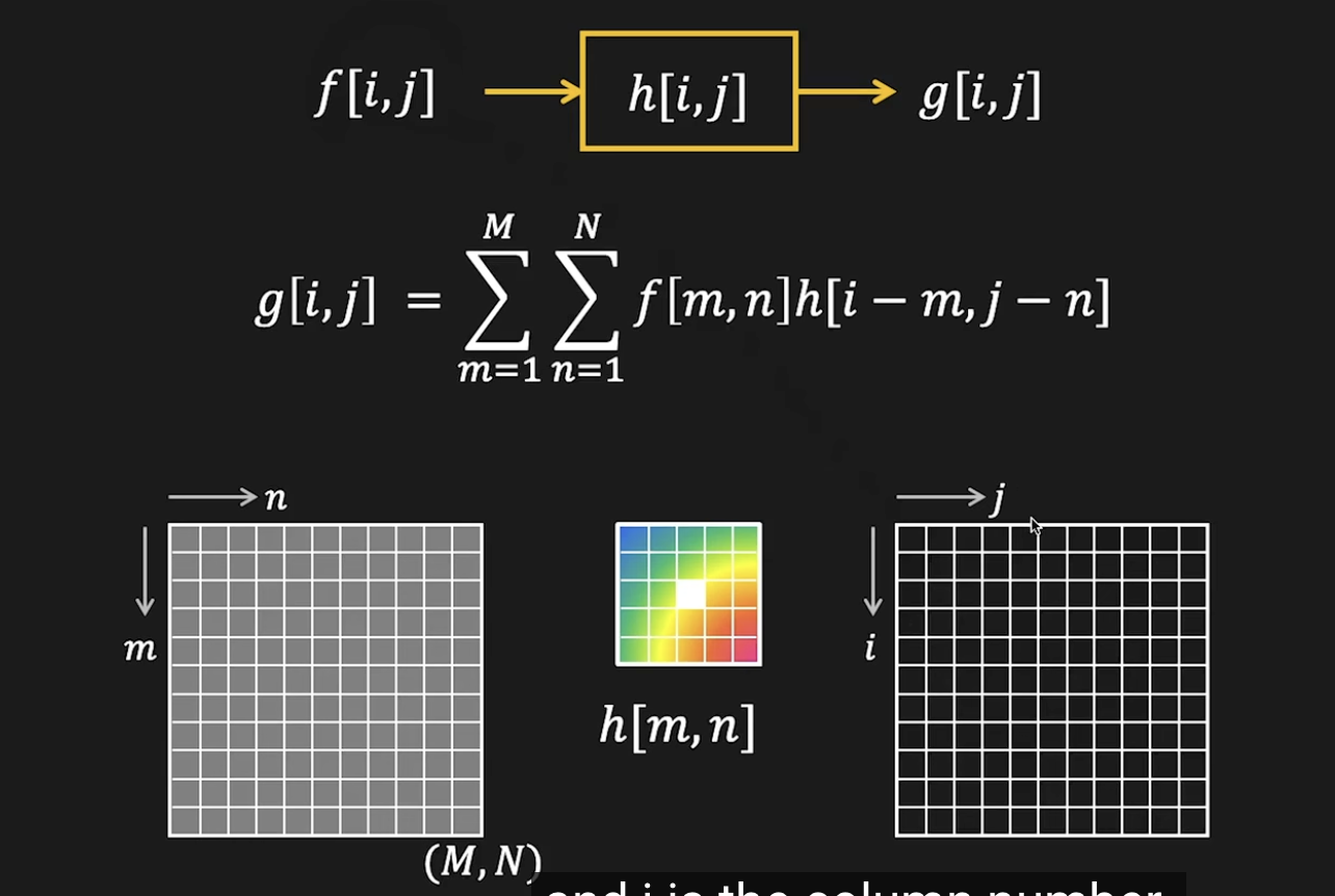
\(h\) is usually called as convolution mask or convolution kernel or convolution filter.
If we want to understand what happen when the kernel is applied to a single pixel, first of all it is flipped twice, then it is applied to the pixel:
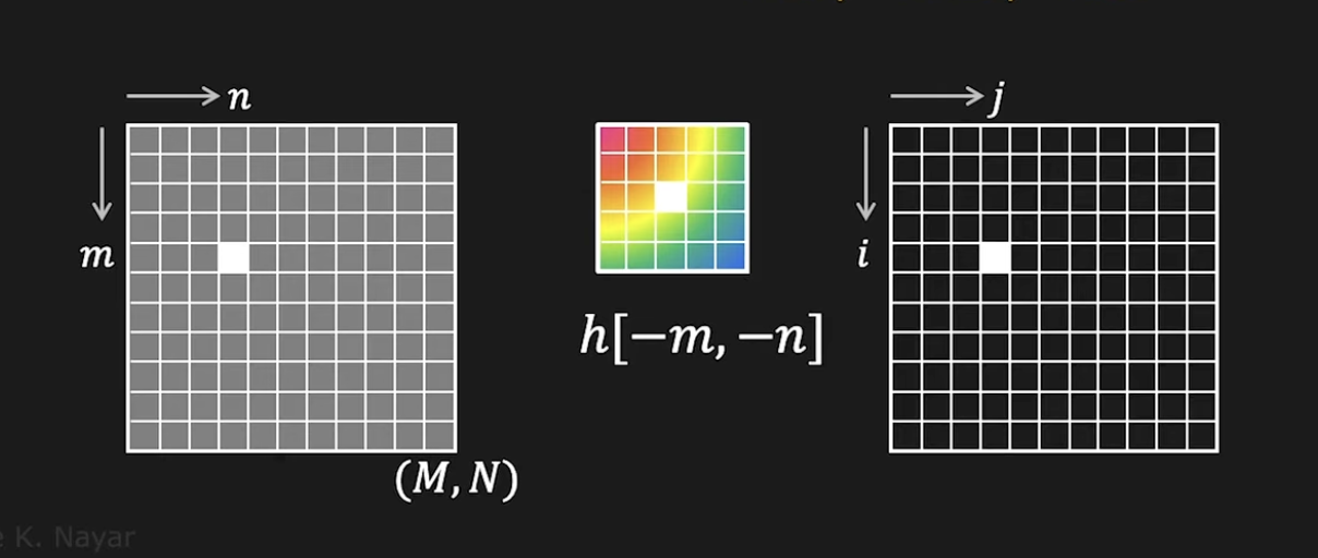
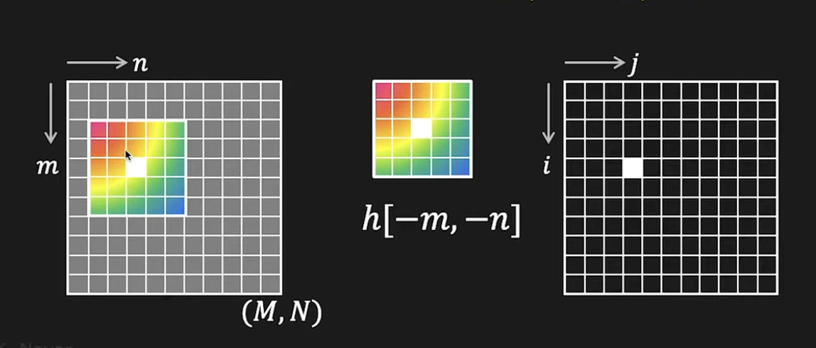
Then you sum all the values and this is the result stored in the output pixel:
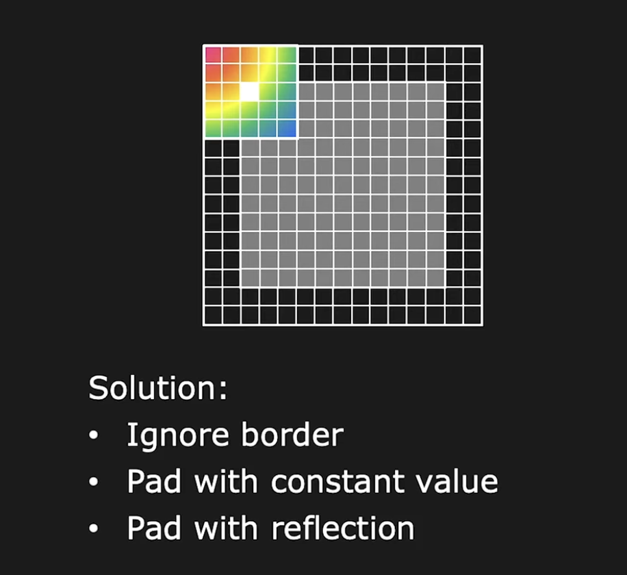
What about the borders? To apply the convolution to a pixel on the border is necessary to extend somehow the image.
Examples
If we convolve with the impulse function, we obtain the sama image of the input:
If we consider the box kernel, as a square of constant value equal to one:
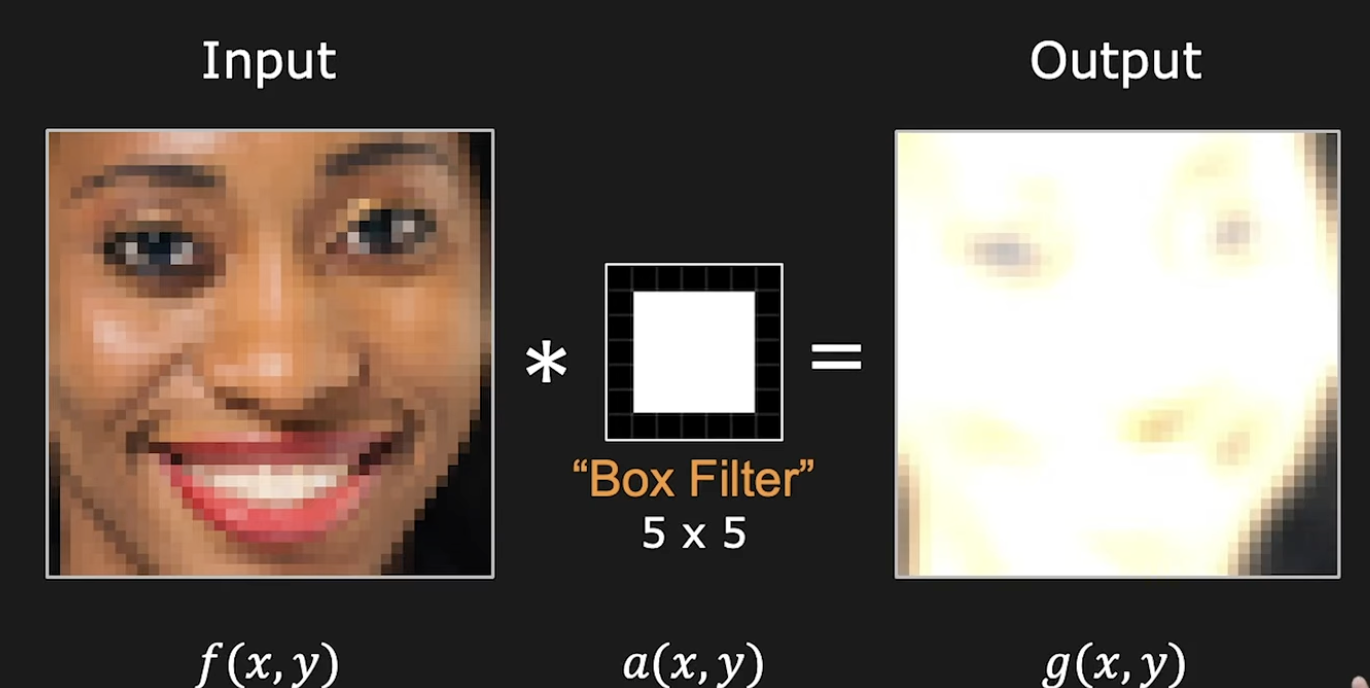
The output image is saturated. If we normalize the values inside the box by diving by the area of the box we obtain:
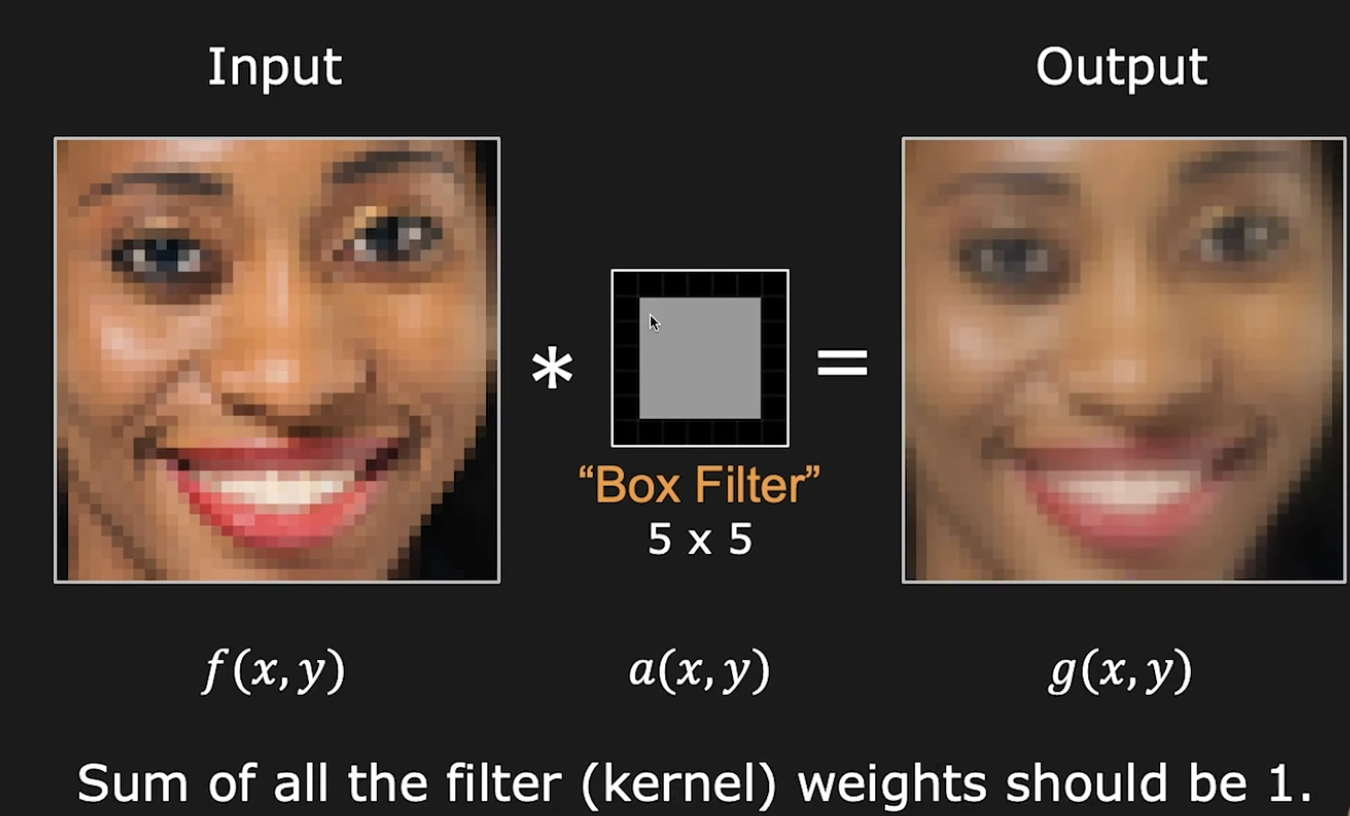
How to improve the results of the box filter where blocky artifacts are visible? With a fuzzy filter:
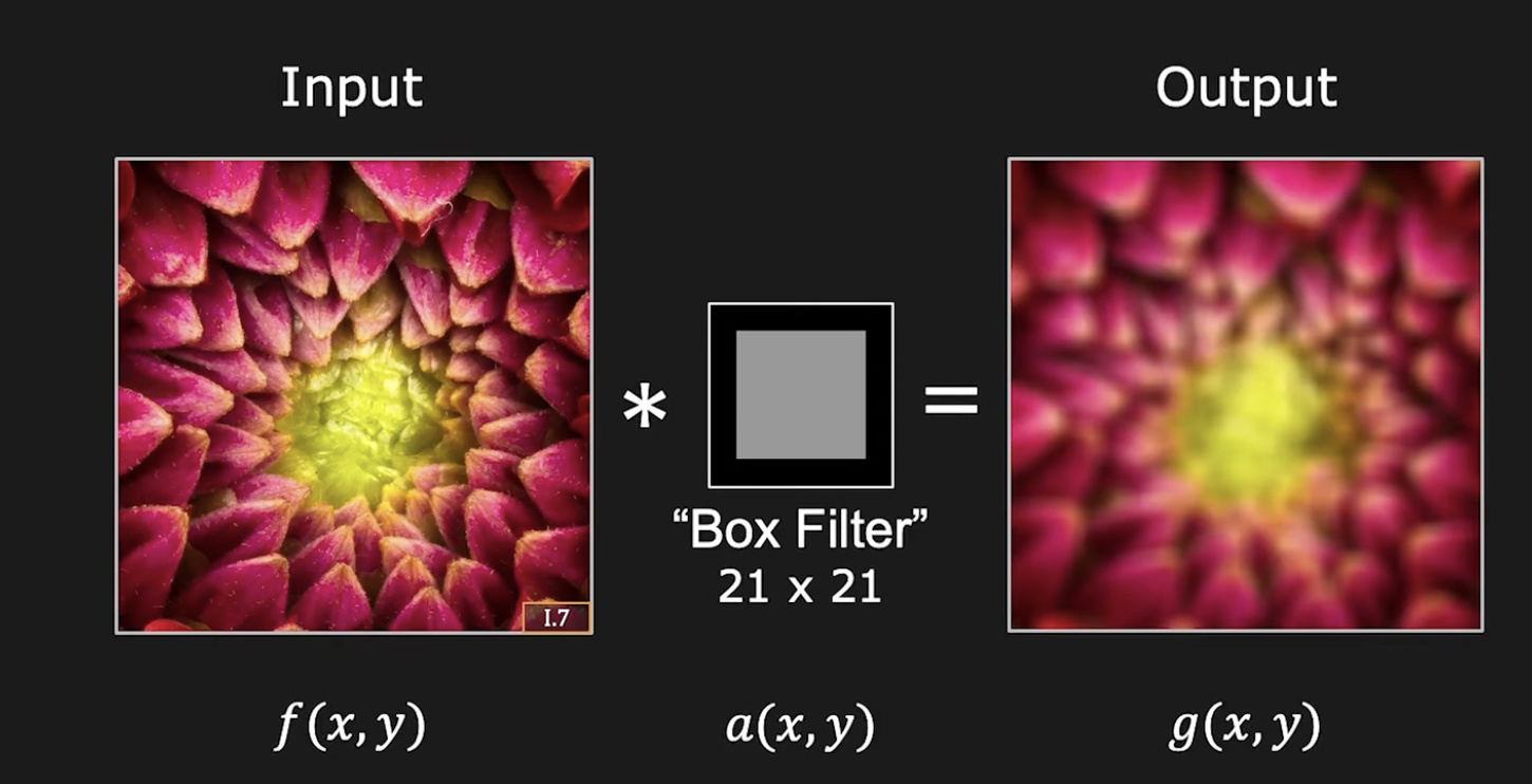
Fig. 5 Box filter 21x21#
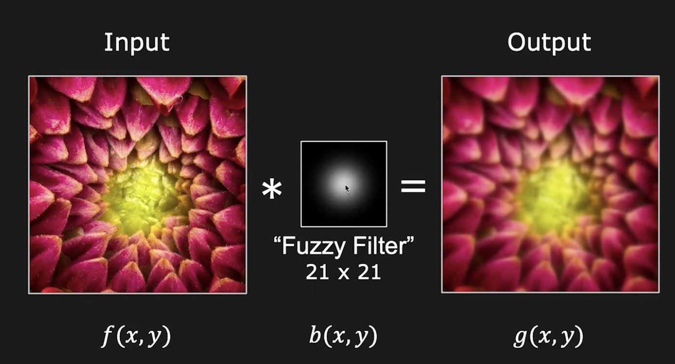
Fig. 6 fuzzy filter 21x21#
The maximum value is in the center and the the values symmetrivally decrease far from the centre. In this case the image is smoothed but there aren’t any more blocky artifacts.
The fuzzy filter can be expressd mathematically by means of the gaussian function.
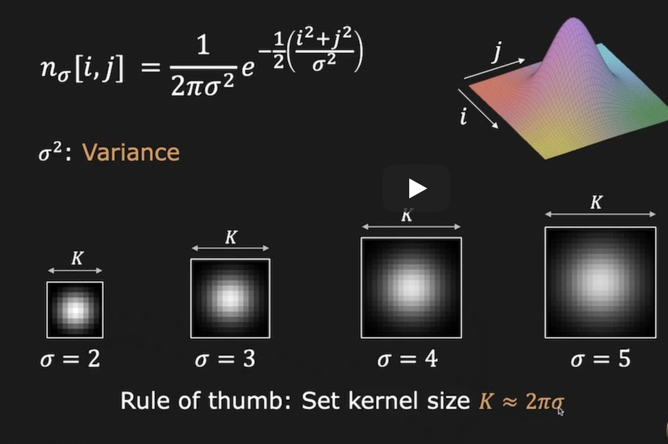
Note that the gaussian function goes to zero only at infinity. Which is the best size of gaussian mask to use? Ususally, \(k \simeq 2 \pi \sigma\). An example:
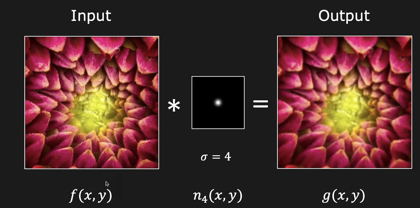
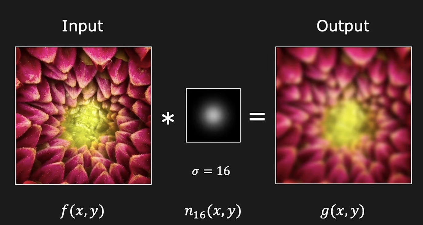
The Gaussian filter has the property to be separable:
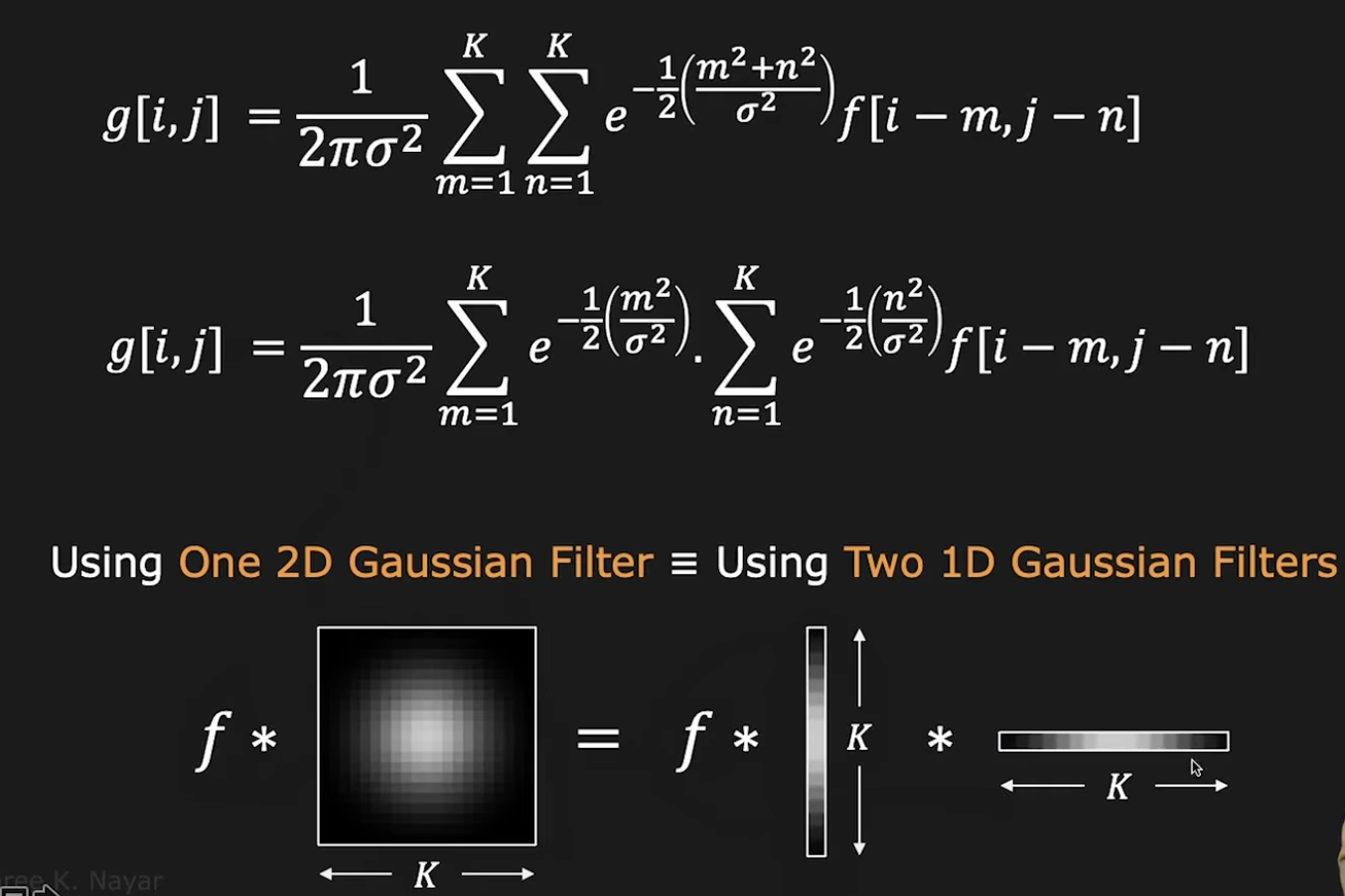
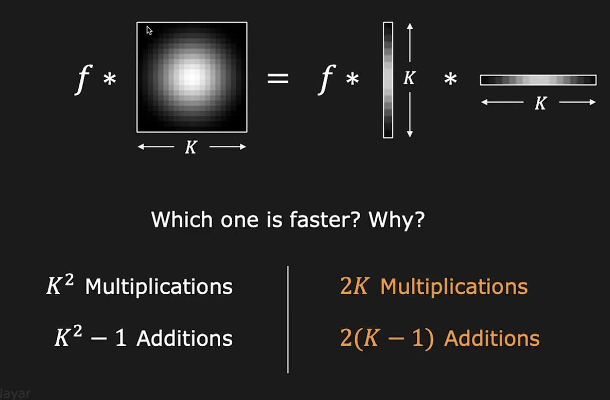
This is important for the computational cost. We can examine the cost for a single pixel. The total cost is obtained by summing the cost for all the pixels in the image.
Non linear filters#
Non linear filters cannot be implemented with convolutions.
Why use non linear filters: An example. We want to remove salt-and-peppers noise froma an image.
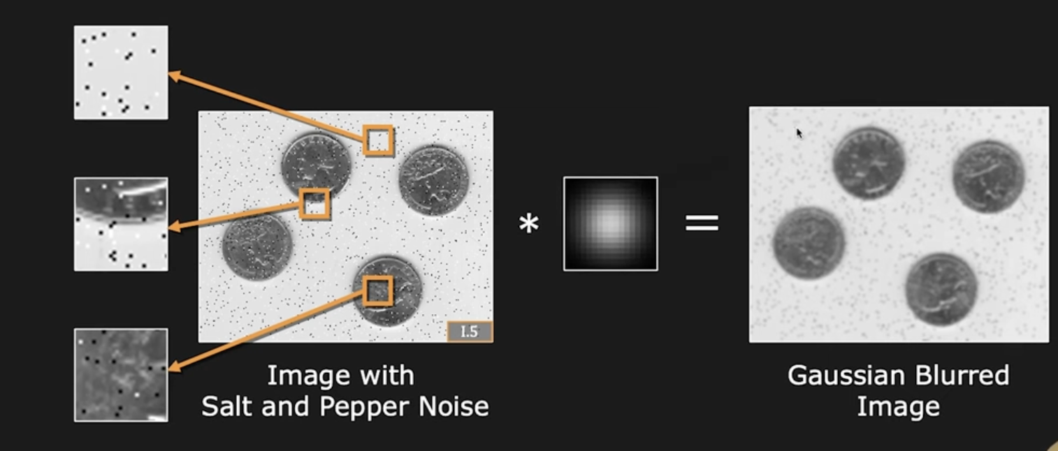
With a gaussian filter the noise is not exactly removed, but smeared out, but we are also loosing some details on the coins.
Median filter
The median filter is obtained by means of this algorithm, for each pixel. 1- Create a square mask around the pixel. 2- sort the values of the pixels n teh mask. 3- Consider the median of that values. 4- subsitute the medianl value to the considered pixel. This is the new value of the pixel in the filtered image.
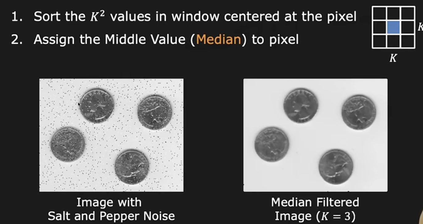
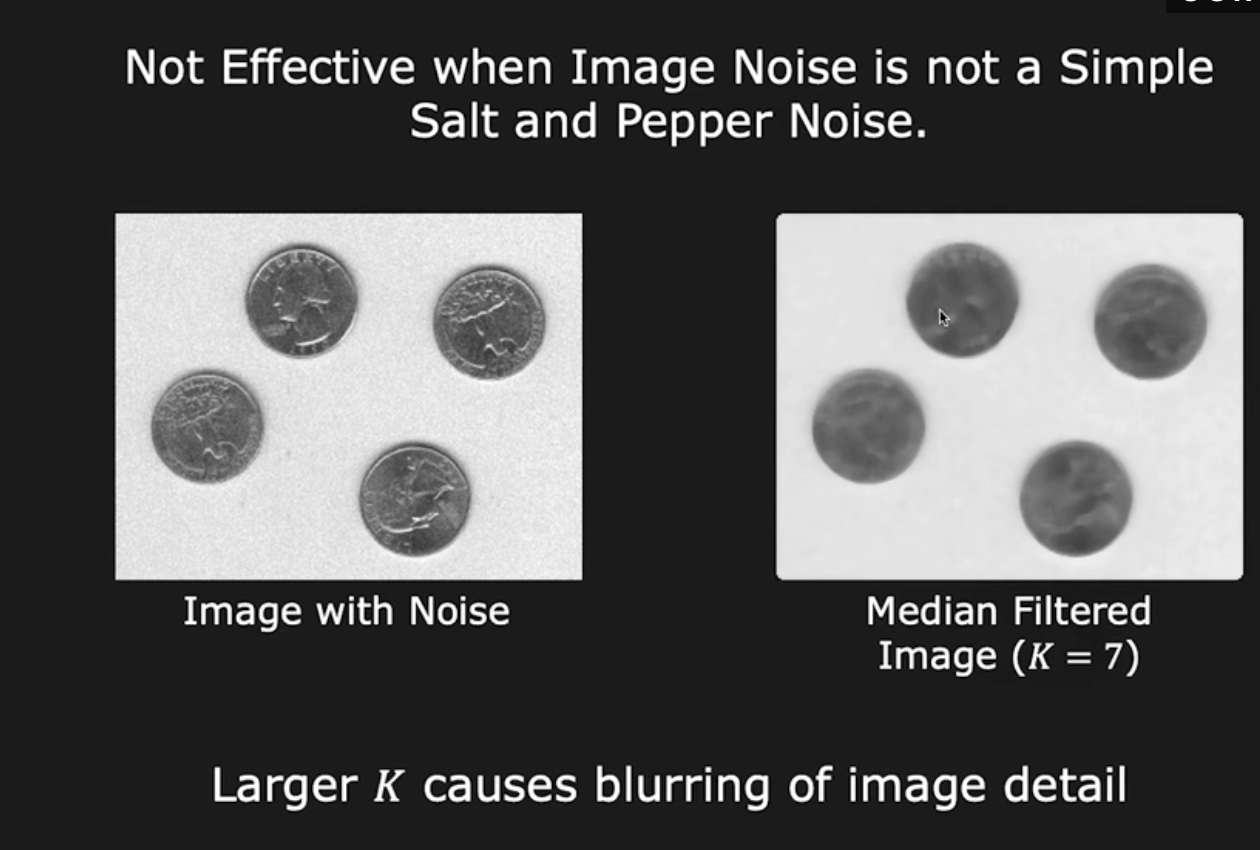
but if you use a larger mask, the noise is better removed but the image is quite blurred:
Bilateral filter
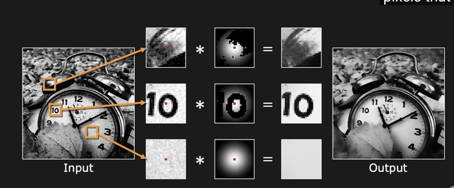
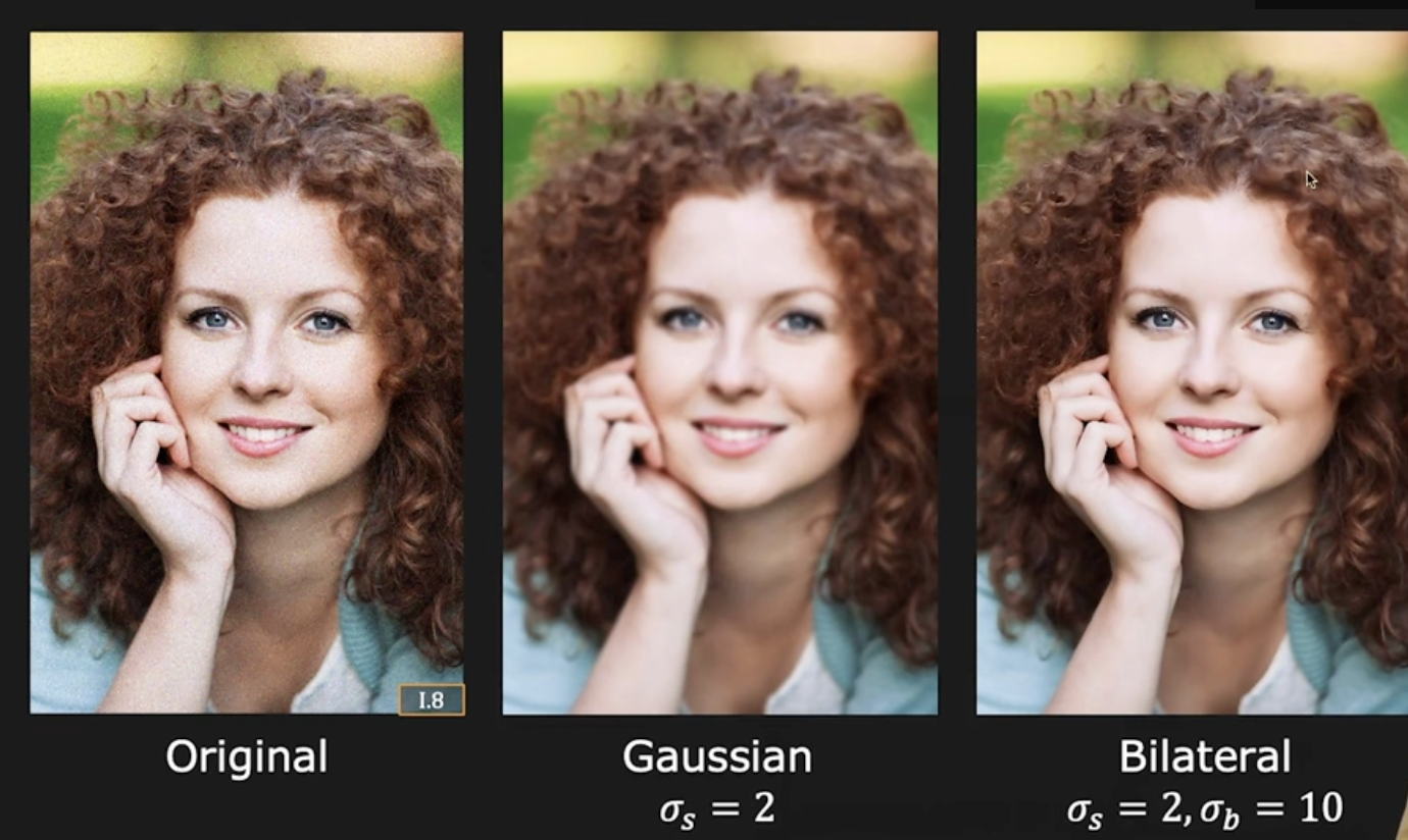
Suppose now to go back to the gaussian filter, but not use the same filter for any pixel. In practice, we want to create a single filter for each pixel, that takes care of the context where the pixel is and of its neighbour pixels. We can, for example, eliminate the pxels that have a too different brightness value from the agussian mask:
How to create a filter like this? If you apply the gaussina filter to an image like a step and youi cneter the filter in the yellow pixels, the red and green pixels have the same smoothing, vene if they are at oppsite sides of the step. the final result is the smoothe image (surface) on the left, that obviously is not satisfactory.
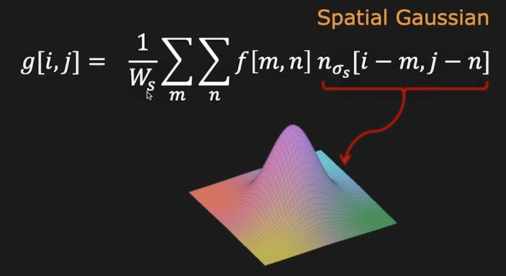
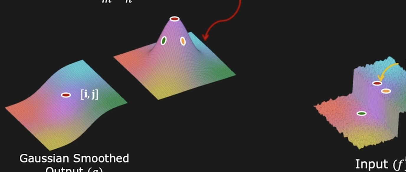
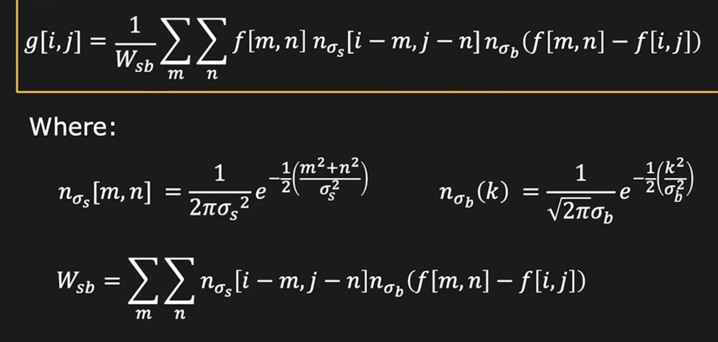
To face this problem, we add a new term to the filter, that is called brightness gaussian that cares abut the brigtness of the pixels in the mask an by means of the coefficent large weights are assigned when the difference of brightness is small and samll weights are assigned when the difference of brightness is large.
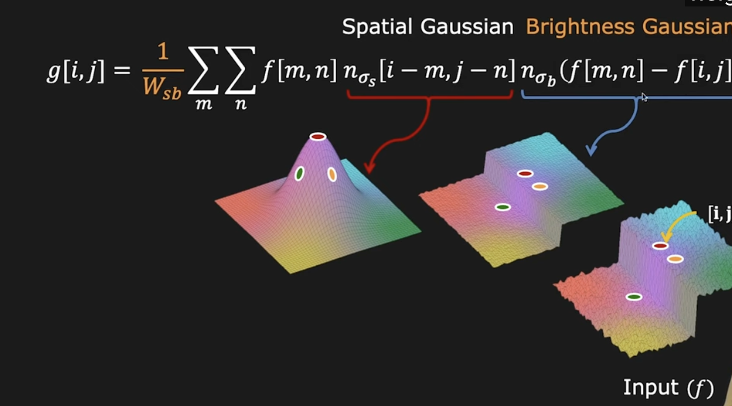
so that the final filters looks like this:
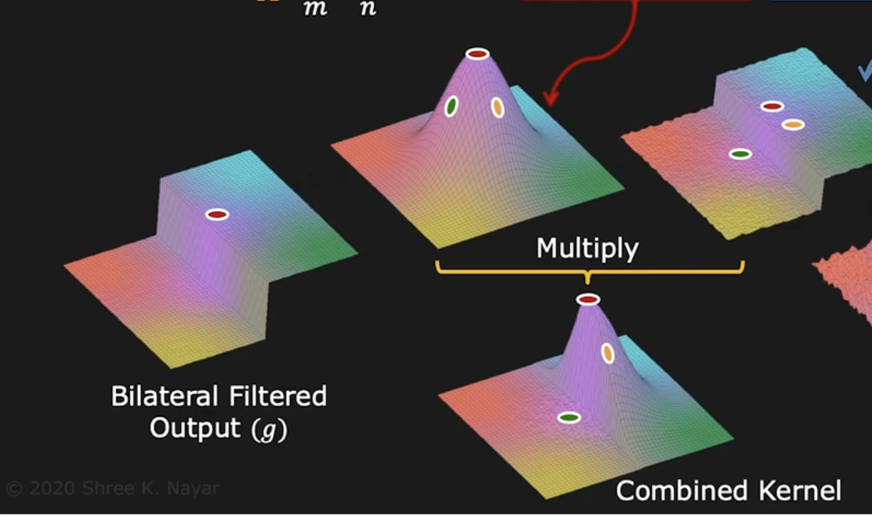
The explicit form of the bilateral filter is the follwing:
Examples:
Increasing \( \sigma \):