Hybrid methods: Plug and Play#

Model Based approach
(+) Take account of the physical (or statistical )model and can incorporate physical (or statistical) priors
(+) Explainability of the results
(-) Choice of the regularization function and regularization parameter
(-) Long execution time
FRom Model based to data driven
Speed and Efficiency
MBIR involves iterative updates, which can be computationally expensive.
Neural networks, once trained, can perform reconstructions in real time, significantly reducing processing times.
Data-Driven Learning
MBIR depends on handcrafted priors and explicit regularization.
Neural networks can automatically learn priors from large datasets, capturing complex image features without manual tuning.
Robustness to Noise
MBIR incorporates statistical noise models, but these may not generalize well across different imaging conditions.
Deep learning models can be trained to handle diverse noise patterns, improving robustness.
End-to-End Optimization
MBIR requires solving multiple steps sequentially (forward model, regularization, optimization).
Neural networks can be trained in an end-to-end fashion, directly mapping raw data to high-quality reconstructions.
Data driven methods
(+) Fast execution after training, the execution is real time
(+) high quality reconstruction since the information is obtained from multiple data
(-) Data Dependency: Large, high-quality datasets are required for training.
(-) Generalization: Neural networks may not always generalize well to unseen data (instability)
(-) Interpretability: MBIR methods offer explicit mathematical formulations, whereas deep learning models often function as black boxes.
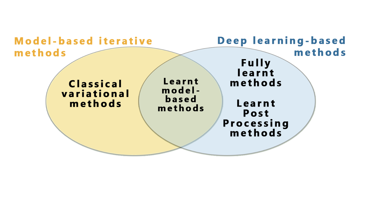
Examples of hybrid methods
Plug and Play - Neural networks learning the denoiser
Bilevel methods - neural networks learn the regularizer
Unrolled methods- neural networks learns the parameters of the model (such as the regularization parameter) of the parameters of the optimization algorithm
Learned Post processing (LPP)- the neural network is used as a post processing of an MBIR method
Other hybrid methods – The neural networks learns some iterations of the iterative method (RISING), the initial guess of an iterative method for non convex minimization, … in general the neural networks are used in the most critical steps of an MBIR approach.
The Plug and Play approach
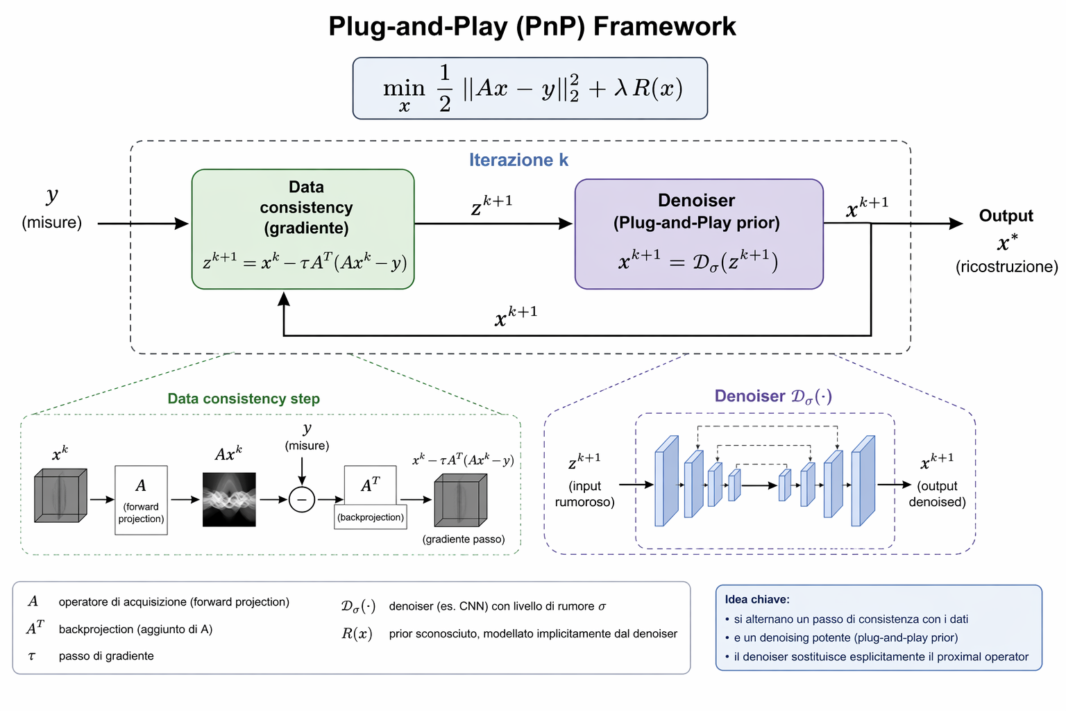
The Plug and Play (PnP) framework incorporates advanced prior models.
It’s fundamental goal is to fuse the model based apporach with action based models, such as Deep NN (DNN) that are dsigned to generate output from input.
In the PnP prior the prior model is replaced by a general class of denoising operators that can be efficiently Implemented by DNNs.
(Kamilov, Ulugbek S., et al. “Plug-and-play methods for integrating physical and learned models in computational imaging: Theory, algorithms, and applications.” IEEE Signal Processing Magazine 40.1 (2023): 85-97.)
The idea is to decouple the forward model (the physics of the measurement) from the prior (the model of the image):
Where the least squares part represents the fidelity term with the data and \(R(x)\) is the regularization term, \(\lambda\) is a trade off parameter.
The fidelity term guarantees the solution accords with the degradation process, while the regularization term enforces desired properties of the output.
Generally, the methods to solve the minimization problem can be divided into two main categories, i.e., model-based optimization methods and discriminative learning methods.
The model-based optimization methods aim to directly solve the minimization problem with some optimization algorithms which usually involve a time-consuming iterative inference. On the contrary, discriminative learning methods try to learn the prior parameters and a compact inference through an optimization of a loss function on a training set containing degraded-clean image pairs.
It can be seen that one obvious difference between model-based optimization method and discriminative learning method is that, the former is flexible to handle various IR tasks by specifying degradation matrix H, whereas the latter needs to use the training data with certain degradation matrices to learn the model.
As a consequence, different from model-based optimization methods which have flexibility to handle different image restoration tasks, discriminative learning methods are usually restricted by specialized tasks.
With the sacrifice of flexibility, however, discriminative learning methods can not only enjoy a fast testing speed but also tend to deliver promising performance due to the joint optimization and end-to-end training.
On the contrary, model-based optimization methods are usually time consuming with sophisticated priors for the purpose of good performance.
As a result, those two kinds of methods have their respective merits and drawbacks, and thus it would be attractive to investigate their integration which leverages their respective merits.
Fortunately, with the aid of variable splitting techniques, such as alternating direction method of multipliers (ADMM) method and half quadratic splitting (HQS) method , it is possible to deal with fidelity term and regularization term separately , and particularly, the regularization term only corresponds to a denoising subproblem.

The Half Quadratic Splitting (HQS) algorithm
Conoder the previous model:
By introducing an auxiliary variable z, the Half Quadratic Splitting (HQS) method tries to solve the constrained problem:
This is equivalent to solve:
where \(\mu\) is a penalty parameter.
The minimization problem is solved by means of the following splitting scheme:
Where the fidelity and the regularization term are decoupled into two different equations.
The first equation is a Tikhonov regularization problem can be solved with a suitable method. The second equation represents the denoising of the image \(x_{k+1}\). A denoiser can be plugged in.
Algorithm
for k=1,2,..
\( \ \ z_{k+1}=D^{CNN}(x_k)\)
\( \ \ x_{k+1}=argmin_x \|Ax-y^{\delta}\|_2^2+\mu \|x-z_{k+1}\|_2^2\)
end for
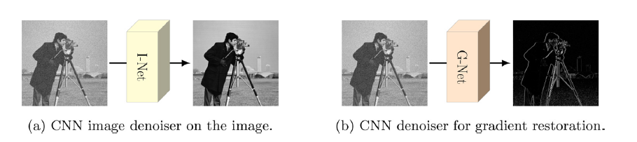
The denoiser \(D^{CNN}\) can be implemented by a neural network.
The neural network can be for example a Residual Unet that is trained from low dose
noisy sinograms to ground truth.
It is also possible to set up neural networks acting on the gradient \(D\) of the image:
The HQS method in this case reads as:
Now the first equation represents the denoising of Dx, i.e. the image of the gradient of x.
Hence it is possible to plug in a neural network acting as a denoiser on the gradients. A ResUnet can be used, for example with a final layer exctrating the gradients from the output image. Or trained directly on the image gradients starting from the noisy sinograms. More details will be given in the next lessons.
Algorithm
for k=1,2,..
\( \ \ z_{k+1}=D^{CNN}(Dx_k)\)
\( \ \ x_{k+1}=argmin_x \|Ax-y^{\delta}\|_2^2+\mu \|Dx-z_{k+1}\|_2^2\)
end for